
See the pkgdown site at norskregnesentral.github.io/shapr/ for a complete introduction with examples and documentation of the package.
For an overview of the methodology and capabilities of the package (per shapr v1.0.8), see the software paper Jullum et al. (2025), available as a preprint here.
NEWS
With shapr version 1.0.0 (GitHub only, Nov 2024) and version 1.0.1 (CRAN, Jan 2025), the package underwent a major update, providing a full restructuring of the code base, and a full suite of new functionality, including:
- A long list of approaches for estimating the contribution/value function , including Variational Autoencoders and regression-based methods
- Iterative Shapley value estimation with convergence detection
- Parallelized computations with progress updates
- Reweighted Kernel SHAP for faster convergence
- New function
explain_forecast()for explaining forecasts - Asymmetric and causal Shapley values
- Several other methodological, computational and user-experience improvements
- Python wrapper
pyshaprmaking the core functionality ofshapravailable in Python
See the NEWS for a complete list.
Coming from shapr < 1.0.0?
shapr version >= 1.0.0 comes with a number of breaking changes. Most notably, we moved from using two functions (shapr() and explain()) to one function (explain()). In addition, custom models are now explained by passing the prediction function directly to explain(). Several input arguments were renamed, and a few functions for edge cases were removed to simplify the code base.
Click here to view a version of this README with the old syntax (v0.2.2).
Python wrapper
We provide a Python wrapper (pyshapr) which allows explaining Python models with the methodology implemented in shapr, directly from Python. The wrapper calls R internally and therefore requires an installation of R. See here for installation instructions and examples.
The package
The shapr R package implements an enhanced version of the Kernel SHAP method for approximating Shapley values, with a strong focus on conditional Shapley values. The core idea is to remain completely model-agnostic while offering a variety of methods for estimating contribution functions, enabling accurate computation of conditional Shapley values across different feature types, dependencies, and distributions. The package also includes evaluation metrics to compare various approaches. With features like parallelized computations, convergence detection, progress updates, and extensive plotting options, shapr is a highly efficient and user-friendly tool, delivering precise estimates of conditional Shapley values, which are critical for understanding how features truly contribute to predictions. In addition to local prediction explanations, shapr also supports global feature importance through SAGE (Shapley Additive Global importancE) values, computed by setting scope = "global" in explain().
A basic example is provided below. Otherwise, we refer to the pkgdown website and the vignettes there for details and further examples.
Installation
shapr is available on CRAN and can be installed in R as:
install.packages("shapr")To install the development version of shapr, available on GitHub, use
remotes::install_github("NorskRegnesentral/shapr")To also install all dependencies, use
remotes::install_github("NorskRegnesentral/shapr", dependencies = TRUE)Example
shapr supports computation of Shapley values with any predictive model that takes a set of numeric features and produces a numeric outcome.
The following example shows how a simple xgboost model is trained using the airquality dataset, and how shapr explains the individual predictions.
We first enable parallel computation and progress updates with the following code chunk. These are optional, but recommended for improved performance and user-friendliness, particularly for problems with many features.
# Enable parallel computation
# Requires the future and future_lapply packages
future::plan("multisession", workers = 2) # Increase the number of workers for increased performance with many features

# Enable progress updates of the v(S) computations
# Requires the progressr package
progressr::handlers(global = TRUE)
progressr::handlers("cli") # Using the cli package as backend (recommended for the estimates of the remaining time)
Here is the actual example:
library(xgboost)
library(shapr)

data("airquality")
data <- data.table::as.data.table(airquality)
data <- data[complete.cases(data), ]

x_var <- c("Solar.R", "Wind", "Temp", "Month")
y_var <- "Ozone"

ind_x_explain <- 1:6
x_train <- data[-ind_x_explain, ..x_var]
y_train <- data[-ind_x_explain, get(y_var)]
x_explain <- data[ind_x_explain, ..x_var]

# Look at the dependence between the features
cor(x_train)
#>            Solar.R       Wind       Temp      Month
#> Solar.R  1.0000000 -0.1243826  0.3333554 -0.0710397
#> Wind    -0.1243826  1.0000000 -0.5152133 -0.2013740
#> Temp     0.3333554 -0.5152133  1.0000000  0.3400084
#> Month   -0.0710397 -0.2013740  0.3400084  1.0000000

# Fit a basic xgboost model to the training data
model <- xgboost(
  x = x_train,
  y = y_train,
  nround = 20,
  verbosity = 0
)

# Specify phi_0, i.e., the expected prediction without any features
p0 <- mean(y_train)

# Compute Shapley values with Kernel SHAP, accounting for feature dependence using
# the empirical (conditional) distribution approach with bandwidth parameter sigma = 0.1 (default)
explanation <- explain(
  model = model,
  x_explain = x_explain,
  x_train = x_train,
  approach = "empirical",
  phi0 = p0,
  seed = 1
)
#>
#> ── Starting `shapr::explain()` at 2026-07-06 15:16:23 ──────────────────────────
#> ℹ `max_n_coalitions` is `NULL` or larger than `2^n_features = 16`, and is
#>   therefore set to `2^n_features = 16`.
#>
#>
#> ── Explanation overview ──
#>
#>
#>
#> • Model class: <xgboost>
#>
#> • v(S) estimation class: Monte Carlo integration
#>
#> • Approach: empirical
#>
#> • Procedure: Non-iterative
#>
#> • Number of Monte Carlo integration samples: 1000
#>
#> • Number of feature-wise Shapley values: 4
#>
#> • Number of observations to explain: 6
#>
#> • Computations (temporary) saved at:
#> '/tmp/RtmpJjhNN2/shapr_obj_2cd6d57a3dbee.rds'
#>
#>
#>
#> ── Main computation started ──
#>
#>
#>
#> ℹ Using 16 of 16 coalitions.

# Print the Shapley values for the observations to explain.
print(explanation)
#>    explain_id  none Solar.R   Wind   Temp  Month
#>         <int> <num>   <num>  <num>  <num>  <num>
#> 1:          1  43.1  12.315   2.78 -27.98  -2.07
#> 2:          2  43.1  -8.514   4.69 -13.96  -7.85
#> 3:          3  43.1  -2.767 -10.27  -9.95  -3.87
#> 4:          4  43.1  -0.945  -4.18 -14.06  -6.80
#> 5:          5  43.1   4.058  -2.07 -11.94 -12.02
#> 6:          6  43.1  -0.290  -7.28 -13.46  -6.50

# Provide a formatted summary of the shapr object
summary(explanation)
#>
#> ── Summary of Shapley value explanation ────────────────────────────────────────
#> • Computed with `shapr::explain()` in 2.5 seconds, started 2026-07-06 15:16:23
#> • Model class: <xgboost>
#> • v(S) estimation class: Monte Carlo integration
#> • Approach: empirical
#> • Procedure: Non-iterative
#> • Number of Monte Carlo integration samples: 1000
#> • Number of feature-wise Shapley values: 4
#> • Number of observations to explain: 6
#> • Number of coalitions used: 16 (of total 16)
#> • Computations (temporary) saved at:
#> '/tmp/RtmpJjhNN2/shapr_obj_2cd6d57a3dbee.rds'
#>
#> ── Estimated Shapley values
#>    explain_id   none Solar.R   Wind   Temp  Month
#>         <int> <char>  <char> <char> <char> <char>
#> 1:          1  43.09   12.31   2.78 -27.98  -2.07
#> 2:          2  43.09   -8.51   4.69 -13.96  -7.85
#> 3:          3  43.09   -2.77 -10.27  -9.95  -3.87
#> 4:          4  43.09   -0.95  -4.18 -14.06  -6.80
#> 5:          5  43.09    4.06  -2.07 -11.94 -12.02
#> 6:          6  43.09   -0.29  -7.28 -13.46  -6.50
#> ── Estimated MSEv
#> Estimated MSE of v(S) = 208 (with sd = 116)

# Finally, we plot the resulting explanations
plot(explanation)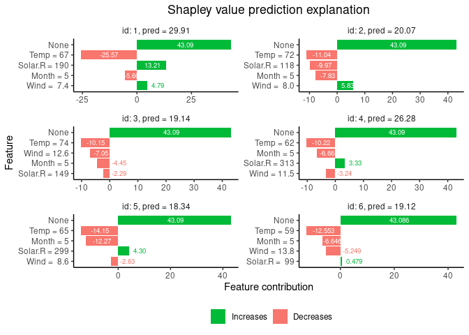
In addition to explaining individual predictions, shapr can compute global feature importance through SAGE (Shapley Additive Global importancE) values by setting scope = "global" and providing the observed responses via y_explain. The loss defaults to log-loss for binary 0/1 responses and the mean squared error otherwise, and a custom loss can be supplied through extra_computation_args$global_loss_func.
# Compute SAGE values explaining the model's global loss (MSE by default)
sage_explanation <- explain(
  model = model,
  x_explain = x_explain,
  x_train = x_train,
  approach = "empirical",
  phi0 = p0,
  scope = "global",
  y_explain = data[ind_x_explain, get(y_var)],
  seed = 1
)
#>
#> ── Starting `shapr::explain()` at 2026-07-06 15:16:29 ──────────────────────────
#> ℹ `max_n_coalitions` is `NULL` or larger than `2^n_features = 16`, and is
#>   therefore set to `2^n_features = 16`.
#>
#>
#> ── Explanation overview ──
#>
#>
#>
#> • Model class: <xgboost>
#>
#> • v(S) estimation class: Monte Carlo integration
#>
#> • Approach: empirical
#>
#> • Procedure: Non-iterative
#>
#> • Number of Monte Carlo integration samples: 1000
#>
#> • Number of feature-wise Shapley values: 4
#>
#> • Number of observations to explain: 6
#>
#> • Computations (temporary) saved at:
#> '/tmp/RtmpJjhNN2/shapr_obj_2cd6d2777ad60.rds'
#>
#>
#>
#> ── Main computation started ──
#>
#>
#>
#> ℹ Using 16 of 16 coalitions.

# Print the SAGE values
print(sage_explanation)
#>    explain_id  none Solar.R  Wind  Temp Month
#>         <int> <num>   <num> <num> <num> <num>
#> 1:          1  -439   -49.3   174   166  58.4

# Plot the SAGE values as a bar chart
plot(sage_explanation, plot_type = "bar")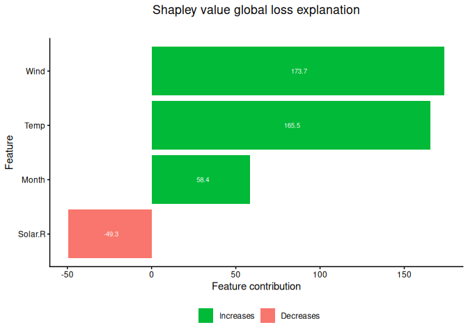
See Jullum et al. (2025) (preprint available here) for a software paper with an overview of the methodology and capabilities of the package (as of v1.0.8). See the general usage vignette for further basic usage examples and brief introductions to the methodology. For more thorough information about the underlying methodology, see methodological papers Aas, Jullum, and Løland (2021), Redelmeier, Jullum, and Aas (2020), Jullum, Redelmeier, and Aas (2021), Olsen et al. (2022), Olsen et al. (2024) and Olsen and Jullum (2025). See also Sellereite and Jullum (2019) for a very brief paper about a previous version (v0.1.1) of the package (with a different structure, syntax, and significantly less functionality).
Contribution
All feedback and suggestions are very welcome. Details on how to contribute can be found here. If you have any questions or comments, feel free to open an issue here.
Please note that the shapr project is released with a Contributor Code of Conduct. By contributing to this project, you agree to abide by its terms.