Asymmetric and causal Shapley value explanations

Overview

This vignette elaborates and demonstrates the asymmetric and causal Shapley value frameworks introduced by Frye, Rowat, and Feige (2020) and Heskes et al. (2020), respectively. We also consider the marginal and conditional Shapley value frameworks, see Lundberg and Lee (2017) and Aas, Jullum, and Løland (2021), respectively. We demonstrate the frameworks on the bike sharing dataset from the UCI Machine Learning Repository. The setup is based on the CauSHAPley package, which is the code supplement to the Heskes et al. (2020) paper. The CauSHAPley package was based on an old version of shapr and was restricted to the gaussian approach (see section 6 in Heskes et al. (2020) for more details).

We have extended the causal Shapley value framework to work for all Monte Carlo-based approaches (independence (not recommended), empirical, gaussian, copula, ctree, vaeac and categorical), while the extension of the asymmetric Shapley value framework works for all the Monte Carlo and regression-based approaches. Our generalization is of uttermost importance, as many real-world data sets are far from the Gaussian distribution, and, compared to CauSHAPley, our implementation can utilize all of shapr’s new features, such as batch computation, parallelization and iterative computation for both feature-wise and group-wise Shapley values.

The main differences between the marginal, conditional, and casual Shapley value frameworks is that they sample/generate the Monte Carlo samples from the marginal distribution, (conventional) observational conditional distribution, and interventional conditional distribution, respectively. Asymmetric means that we do not consider all possible coalitions, but rather only the coalitions that respects a causal ordering.

Asymmetric conditional Shapley values

Asymmetric (conditional) Shapley values were proposed by Frye, Rowat, and Feige (2020) as a way to incorporate causal knowledge in the real world by computing the Shapley value explanations using only the feature combinations/coalitions consistent with a (partial) causal ordering. See the figure below for a schematic overview of the causal ordering we are going to use in the examples in this vignette. In the figure, we see that our causal ordering consists of three components: $\tau_1 = \{X_1\}$ , $\tau_2 = \{X_2, X_3\}$ , and $\tau_3 = \{X_4, X_5, X_6, X_7\}$ . See the code section for what the features represent.

To elaborate, instead of considering the $2^M$ possible coalitions, where $M$ is the number of features, asymmetric Shapley values only consider the subset of coalitions which respects the causal ordering. For our causal ordering, this means that the asymmetric Shapley value explanation framework skips the coalitions where $X_2$ is included but $X_1$ , as $X_1$ is the ancestor of $X_2$ . This will skew the explanations towards distal/root causes, see Section 3.2 in Frye, Rowat, and Feige (2020).

We can use all approaches in shapr, both Monte Carlo-based and regression based methods, to compute the asymmetric Shapley values. This is because the asymmetric Shapley value explanation framework does not change how we compute the contribution functions $v(S)$ , but rather which of the coalitions $S$ that are used to compute the Shapley value explanations. This means that the number of coalitions are no longer $O(2^M)$ , but rather $O(2^{\tau_0})$ , where $\tau_0 = \operatorname{max}_i |\tau_i|$ is the number of features ( $|\tau_i|$ ) in the largest component of the causal ordering.

Furthermore, asymmetric Shapley values supports groups of features, but then the causal ordering must be given on the group level instead of on the feature level. The asymmetric Shapley value framework also supports sampling of coalitions where the sampling is done from the set of coalitions that respects the causal ordering.

Finally, we want make a remark that asymmetric conditional Shapley values are equivalent to asymmetric causal Shapley values (see below) when we only use the coalitions respecting the causal ordering and assuming that all dependencies within chain components are induced by mutual interactions.

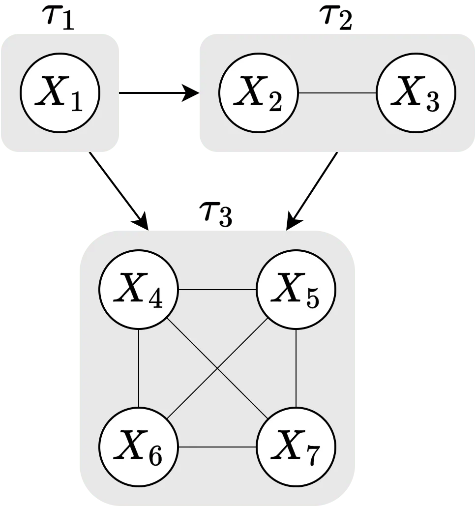
Schematic overview of the causal ordering used in this vignette.

Causal Shapley values

Causal Shapley values were proposed by Heskes et al. (2020) as a way to explain the total effect of features on the prediction by taking into account their causal relationships and adapting the sampling procedure in shapr. More precisely, they propose to employ Pearl’s do-calculus to circumvent the independence assumption, made by Lundberg and Lee (2017), without sacrificing any of the desirable properties of the Shapley value framework. The causal Shapley value explanation framework can also separate the contribution of direct and indirect effects, which makes them principally different from marginal and conditional Shapley values. The framework also provides a more direct and robust way to incorporate causal knowledge, compared to the asymmetric Shapley value explanation framework.

To compute causal Shapley values, we have to specify a (partial) causal ordering and make an assumption about the confounding in each component. Together, they form a causal chain graph which contains directed and undirected edges. All features that are treated on an equal footing are linked together with undirected edges and become part of the same chain component. Edges between chain components are directed and represent causal relationships. In the figure below, we have the same causal ordering as above, but we have in addition made the assumption that we have confounding in the second component, but no confounding in the first and third components. This allows us to correctly distinguishes between dependencies that are due to confounding and mutual interactions. That is, in the figure, the dependencies in chain component $\tau_2$ are assumed to be the result of a common confounder, and those in $\tau_3$ of mutual interactions, while we have no mutual interactions in $\tau_1$ as it is a singleton.

Computing the effect of an intervention depends on how we interpret the generative process that lead to the feature dependencies within each component. If they are the result of marginalizing out a common confounder, then intervention on a particular feature will break the dependency with the other features, and we denote the set of these chain components by $\mathcal{T}_{\text{confounding}}$ . For the components with mutual feature interactions, setting the value of a feature effects the distribution of the variables within the same component. We denote the set of these components by $\mathcal{T}_{\,\overline{\text{confounding}}}$ .

Heskes et al. (2020) described how any expectation by intervention needed to compute the causal Shapley values can be translated to an expectation by observation, by using the interventional formula for causal chain graphs: $\begin{align} \label{eq:do} P(X_{\bar{\mathcal{S}}} \mid do(X_\mathcal{S} = x_\mathcal{S})) = & \prod_{\tau \in \mathcal{T}_{\,\text{confounding}}} P(X_{\tau \cap \bar{\mathcal{S}}} \mid X_{\text{pa}(\tau) \cap \bar{\mathcal{S}}}, x_{\text{pa}(\tau) \cap \mathcal{S}}) \times \tag{1} \\ & \quad \prod_{\tau \in \mathcal{T}_{\,\overline{\text{confounding}}}} P(X_{\tau \cap \bar{\mathcal{S}}} \mid X_{\text{pa}(\tau) \cap \bar{\mathcal{S}}}, x_{\text{pa}(\tau) \cap \mathcal{S}}, x_{\tau \cap \mathcal{S}}). \end{align}$ Here, any of the Monte Carlo-based approaches in shapr can be used to compute the conditional distributions/observational expectations. The marginals are estimated from the training data for all approaches except gaussian, for which we use the marginals of the Gaussian distribution instead.

For specific causal chain graphs, the causal Shapley value framework simplifies to symmetric conditional, asymmetric conditional, and marginal Shapley values, see Corollary 1 to 3 in the supplement of Heskes et al. (2020).

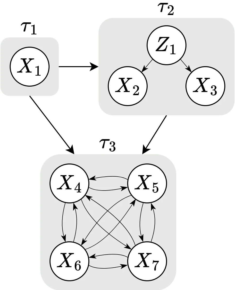
Schematic overview of the causal chain graph used in this vignette.

Marginal Shapley values

Causal Shapley values are equivalent to marginal Shapley values when all $M$ features are combined into a single component $\tau = \mathcal{M} = \{1,2,...,M\}$ and all dependencies are induced by confounding. Then $\text{pa}(\tau) = \emptyset$ , and $P(X_{\bar{\mathcal{S}}} \mid do(X_\mathcal{S} = x_\mathcal{S}))$ in Equation () simplifies to $P(X_{\bar{\mathcal{S}}} \mid do(X_\mathcal{S} = x_\mathcal{S})) = P(X_{\bar{\mathcal{S}}})$ , as specified in Lundberg and Lee (2017).

The Monte Carlo samples for the marginals are generated by sampling from the training data, except for the gaussian approach where we use the marginals of the estimated multivariate Gaussian distribution. This means that for all other approaches, this is the same as using the independence approach in the conditional Shapley value explanation framework.

Symmetric conditioal Shapley values

Causal Shapley values are equivalent to symmetric conditional Shapley values when all $M$ features are combined in a single component $\tau = \mathcal{M} = \{1,2,...,M\}$ and all dependencies are induced by mutual interaction. Then $\text{pa}(\tau) = \emptyset$ , and $P(X_{\bar{\mathcal{S}}} \mid do(X_\mathcal{S} = x_\mathcal{S}))$ in Equation () simplifies to $P(X_{\bar{\mathcal{S}}} \mid do(X_\mathcal{S} = x_\mathcal{S})) = P(X_{\bar{\mathcal{S}}} \mid X_\mathcal{S} = x_\mathcal{S})$ , as specified in Aas, Jullum, and Løland (2021). Symmetric means that we consider all coalitions.

Code example

Overview

We demonstrate the frameworks on the bike sharing dataset from the UCI Machine Learning Repository. We let the features be the number of days since January 2011 (trend), two cyclical variables representing the season (cosyear, sinyear), temperature (temp), feeling temperature (atemp), wind speed (windspeed), and humidity (hum). The first three features are considered to be a potential cause of the four weather-related features. The bike rental is strongly seasonal and shows an upward trend, as illustrated in the figure below. The bike data is split randomly into a training (80%) and test/explicand (20%) set. We train an XGBoost model for 100 rounds with default variables to act as the model we want to explain.

In the table below, we highlight the Shapley value explanation frameworks introduced above and how to access them by changing the arguments asymmetric, ordering, and confounding in shapr::explain(). Note that symmetric conditional Shapley values are the default version, i.e., by default asymmetric = FALSE, ordering = NULL, confounding = NULL.

Framework	Sampling	Approaches	`asymmetric`	`ordering`	`confounding`
Sym. Conditional	$P(X_{\bar{\mathcal{S}}} \mid (X_\mathcal{S} = x_\mathcal{S})$	All	`FALSE`	`NULL`	`NULL`
Asym. Conditional	$P(X_{\bar{\mathcal{S}}} \mid (X_\mathcal{S} = x_\mathcal{S})$	All	`TRUE`	`list(...)`	`NULL`
Sym. Causal	$P(X_{\bar{\mathcal{S}}} \mid do(X_\mathcal{S} = x_\mathcal{S}))$	All MC-based	`FALSE`	`list(...)`	`c(...)`
Asym. Causal	$P(X_{\bar{\mathcal{S}}} \mid do(X_\mathcal{S} = x_\mathcal{S}))$	All MC-based	`TRUE`	`list(...)`	`c(...)`
Sym. Marginal	$P(X_{\bar{\mathcal{S}}})$	`indep.`, `gaussian`	`FALSE`	`NULL`	`TRUE`

Code setup

First, we load the needed libraries, set up the training/explicand data, plot the data, and train an xgboost model.

library(ggplot2)
library(xgboost)
library(data.table)
library(shapr)

# Additional packages which are only used for plotting in this vignette.
# There are not listed as dependencies is shapr
library(GGally)
library(ggpubr)
library(gridExtra)



# Ensure that shapr's functions are prioritzed, otherwise we need to use the `shapr::`
# prefix when calling explain(). The `conflicted` package is imported by `tidymodels`.
conflicted::conflicts_prefer(shapr::explain, shapr::prepare_data)

# Set up the data
# Can also download the data set from the source https://archive.ics.uci.edu/dataset/275/bike+sharing+dataset
# temp <- tempfile()
# download.file("https://archive.ics.uci.edu/static/public/275/bike+sharing+dataset.zip", temp)
# bike <- read.csv(unz(temp, "day.csv"))
# unlink(temp)
bike <- read.csv("../inst/extdata/day.csv")
# Difference in days, which takes DST into account
bike$trend <- as.numeric(difftime(bike$dteday, bike$dteday[1], units = "days"))
bike$cosyear <- cospi(bike$trend / 365 * 2)
bike$sinyear <- sinpi(bike$trend / 365 * 2)
# Unnormalize variables (see data set information in link above)
bike$temp <- bike$temp * (39 - (-8)) + (-8)
bike$atemp <- bike$atemp * (50 - (-16)) + (-16)
bike$windspeed <- 67 * bike$windspeed
bike$hum <- 100 * bike$hum

# Plot the data
ggplot(bike, aes(x = trend, y = cnt, color = temp)) +
  geom_point(size = 0.75) +
  scale_color_gradient(low = "blue", high = "red") +
  labs(colour = "temp") +
  xlab("Days since 1 January 2011") +
  ylab("Number of bikes rented") +
  theme_minimal() +
  theme(legend.position = "right", legend.title = element_text(size = 10))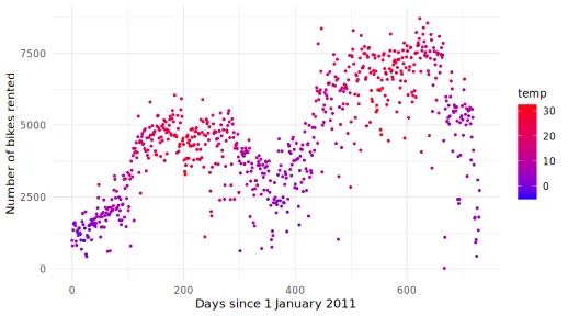

# Define the features and the response variable
x_var <- c("trend", "cosyear", "sinyear", "temp", "atemp", "windspeed", "hum")
y_var <- "cnt"

# NOTE: To avoid RNG reproducibility issues across different systems, we
# load the training-test split from a file. 80% training and 20% test
train_index <- readRDS("../inst/extdata/train_index.rds")

# Training data
x_train <- as.matrix(bike[train_index, x_var])
y_train_nc <- as.matrix(bike[train_index, y_var]) # not centered
y_train <- y_train_nc - mean(y_train_nc)

# Plot pairs plot
GGally::ggpairs(x_train)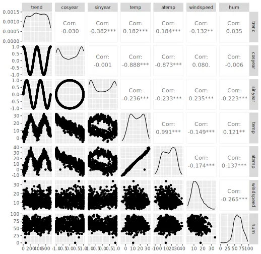

# Test/explicand data
x_explain <- as.matrix(bike[-train_index, x_var])
y_explain_nc <- as.matrix(bike[-train_index, y_var]) # not centered
y_explain <- y_explain_nc - mean(y_train_nc)

# Get 6 explicands to plot the Shapley values of with a wide spread in their predicted outcome
n_index_x_explain <- 6
index_x_explain <- order(y_explain)[seq(1, length(y_explain), length.out = n_index_x_explain)]
y_explain[index_x_explain]
#> [1] -3900.0324 -1872.0324  -377.0324   411.9676  1690.9676  3889.9676

# Fit an XGBoost model to the training data
model <- xgboost::xgboost(
  data = x_train,
  label = y_train,
  nround = 100,
  verbose = FALSE
)

# Save the phi0
phi0 <- mean(y_train)

# Look at the root mean squared error
sqrt(mean((predict(model, x_explain) - y_explain)^2))
#> [1] 798.7148
ggplot(
  data.table("response" = y_explain[, 1], "predicted_response" = predict(model, x_explain)),
  aes(response, predicted_response)
) +
  geom_point()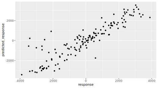

We are going to use the causal_ordering and confounding illustrated in the figures above. For causal_ordering, we can either provide the index of feature or the feature names. Thus, the following two versions of causal_ordering will produce equivalent results. Furthermore, we assume that we have confounding for the second component (i.e., the season has an effect on the weather) and no confounding for the third component (i.e., we do not how to model the intricate relations between the weather features).

causal_ordering <- list(1, c(2, 3), c(4:7))
causal_ordering <- list("trend", c("cosyear", "sinyear"), c("temp", "atemp", "windspeed", "hum"))
confounding <- c(FALSE, TRUE, FALSE)

To make the rest of the vignette easier to follow, we create some helper functions that plot and summarize the results of the explanation methods. This code block is optional to understand and can be skipped.

# Extract the MSEv criterion scores and elapsed times
print_MSEv_scores_and_time <- function(explanation_list) {
  res <- as.data.frame(t(sapply(
    explanation_list,
    function(explanation) {
      round(c(
        explanation$MSEv$MSEv$MSEv,
        explanation$MSEv$MSEv$MSEv_sd,
        difftime(explanation$timing$end_time, explanation$timing$init_time, units = "secs")
      ), 2)
    }
  )))
  colnames(res) <- c("MSEv", "MSEv_sd", "Time (secs)")
  return(res)
}

# Print the full time information
print_time <- function(explanation_list) {
  t(sapply(explanation_list, function(explanation) explanation$timing$total_time_secs))
}

# Make beeswarm plots
plot_beeswarms <- function(explanation_list, title = "", ...) {
  # Make the beeswarm plots
  grobs <- lapply(seq(length(explanation_list)), function(explanation_idx) {
    gg <- plot(explanation_list[[explanation_idx]], plot_type = "beeswarm", ...) +
      ggplot2::ggtitle(tools::toTitleCase(gsub("_", " ", names(explanation_list)[[explanation_idx]])))

    # Flip the order such that the features comes in the right order
    gg <- gg +
      ggplot2::scale_x_discrete(limits = rev(levels(gg$data$variable)[levels(gg$data$variable) != "none"]))
  })

  # Get the limits
  ylim <- sapply(grobs, function(grob) ggplot2::ggplot_build(grob)$layout$panel_scales_y[[1]]$range$range)
  ylim <- c(min(ylim), max(ylim))

  # Update the limits
  grobs <- suppressMessages(lapply(grobs, function(grob) grob + ggplot2::coord_flip(ylim = ylim)))

  # Make the combined plot
  gridExtra::grid.arrange(
    grobs = grobs, ncol = 1,
    top = grid::textGrob(title, gp = grid::gpar(fontsize = 18, font = 8))
  )
}

Symmetric conditional Shapley values (default)

We start by demonstrating how to compute symmetric conditional Shapley values. This is the default version in shapr and there is no need to specify the arguments below. However, we have specified them for the sake of clarity. We use the gaussian, ctree, and regression_separate(xgboost with default hyperparameters) approaches, but any other approach can also be used.

# list to store the results
explanation_sym_con <- list()

explanation_sym_con[["gaussian"]] <- explain(
  model = model,
  x_train = x_train,
  x_explain = x_explain,
  approach = "gaussian",
  phi0 = phi0,
  n_MC_samples = 1000,
  asymmetric = FALSE, # Default value (TRUE will give the same since `causal_ordering = NULL`)
  causal_ordering = NULL, # Default value
  confounding = NULL # Default value
)
#> Note: Feature classes extracted from the model contains NA.
#> Assuming feature classes from the data are correct.
#> Success with message:
#> max_n_coalitions is NULL or larger than or 2^n_features = 128, 
#> and is therefore set to 2^n_features = 128.
#> 
#> ── Starting `shapr::explain()` at 2024-11-21 22:40:52 ──────────────────────────────────────────────────────────────────────────────────────────────────────
#> • Model class: <xgb.Booster>
#> • Approach: gaussian
#> • Iterative estimation: TRUE
#> • Number of feature-wise Shapley values: 7
#> • Number of observations to explain: 144
#> • Computations (temporary) saved at: '/tmp/RtmppO00aE/shapr_obj_1c345f7633c6a7.rds'
#> 
#> ── iterative computation started ──
#> 
#> ── Iteration 1 ─────────────────────────────────────────────────────────────────────────────────────────────────────────────────────────────────────────────
#> ℹ Using 13 of 128 coalitions, 13 new.
#> 
#> ── Iteration 2 ─────────────────────────────────────────────────────────────────────────────────────────────────────────────────────────────────────────────
#> ℹ Using 26 of 128 coalitions, 12 new.
#> 
#> ── Iteration 3 ─────────────────────────────────────────────────────────────────────────────────────────────────────────────────────────────────────────────
#> ℹ Using 36 of 128 coalitions, 10 new.
#> 
#> ── Iteration 4 ─────────────────────────────────────────────────────────────────────────────────────────────────────────────────────────────────────────────
#> ℹ Using 38 of 128 coalitions, 2 new.

explanation_sym_con[["ctree"]] <- explain(
  model = model,
  x_train = x_train,
  x_explain = x_explain,
  approach = "ctree",
  phi0 = phi0,
  n_MC_samples = 1000,
  asymmetric = FALSE, # Default value (TRUE will give the same since `causal_ordering = NULL`)
  causal_ordering = NULL, # Default value
  confounding = NULL # Default value
)
#> Note: Feature classes extracted from the model contains NA.
#> Assuming feature classes from the data are correct.
#> Success with message:
#> max_n_coalitions is NULL or larger than or 2^n_features = 128, 
#> and is therefore set to 2^n_features = 128.
#> 
#> ── Starting `shapr::explain()` at 2024-11-21 22:40:58 ──────────────────────────────────────────────────────────────────────────────────────────────────────
#> • Model class: <xgb.Booster>
#> • Approach: ctree
#> • Iterative estimation: TRUE
#> • Number of feature-wise Shapley values: 7
#> • Number of observations to explain: 144
#> • Computations (temporary) saved at: '/tmp/RtmppO00aE/shapr_obj_1c345f338decc8.rds'
#> 
#> ── iterative computation started ──
#> 
#> ── Iteration 1 ─────────────────────────────────────────────────────────────────────────────────────────────────────────────────────────────────────────────
#> ℹ Using 13 of 128 coalitions, 13 new.
#> 
#> ── Iteration 2 ─────────────────────────────────────────────────────────────────────────────────────────────────────────────────────────────────────────────
#> ℹ Using 26 of 128 coalitions, 12 new.
#> 
#> ── Iteration 3 ─────────────────────────────────────────────────────────────────────────────────────────────────────────────────────────────────────────────
#> ℹ Using 36 of 128 coalitions, 10 new.
#> 
#> ── Iteration 4 ─────────────────────────────────────────────────────────────────────────────────────────────────────────────────────────────────────────────
#> ℹ Using 54 of 128 coalitions, 18 new.
#> 
#> ── Iteration 5 ─────────────────────────────────────────────────────────────────────────────────────────────────────────────────────────────────────────────
#> ℹ Using 64 of 128 coalitions, 10 new.

explanation_sym_con[["xgboost"]] <- explain(
  model = model,
  x_train = x_train,
  x_explain = x_explain,
  phi0 = phi0,
  approach = "regression_separate",
  regression.model = parsnip::boost_tree(engine = "xgboost", mode = "regression"),
  asymmetric = FALSE, # Default value (TRUE will give the same as `causal_ordering = NULL`)
  causal_ordering = NULL, # Default value
  confounding = NULL # Default value
)
#> Note: Feature classes extracted from the model contains NA.
#> Assuming feature classes from the data are correct.
#> Success with message:
#> max_n_coalitions is NULL or larger than or 2^n_features = 128, 
#> and is therefore set to 2^n_features = 128.
#> 
#> ── Starting `shapr::explain()` at 2024-11-21 22:41:42 ──────────────────────────────────────────────────────────────────────────────────────────────────────
#> • Model class: <xgb.Booster>
#> • Approach: regression_separate
#> • Iterative estimation: TRUE
#> • Number of feature-wise Shapley values: 7
#> • Number of observations to explain: 144
#> • Computations (temporary) saved at: '/tmp/RtmppO00aE/shapr_obj_1c345f7e5e3fef.rds'
#> 
#> ── iterative computation started ──
#> 
#> ── Iteration 1 ─────────────────────────────────────────────────────────────────────────────────────────────────────────────────────────────────────────────
#> ℹ Using 13 of 128 coalitions, 13 new.
#> 
#> ── Iteration 2 ─────────────────────────────────────────────────────────────────────────────────────────────────────────────────────────────────────────────
#> ℹ Using 26 of 128 coalitions, 12 new.
#> 
#> ── Iteration 3 ─────────────────────────────────────────────────────────────────────────────────────────────────────────────────────────────────────────────
#> ℹ Using 36 of 128 coalitions, 10 new.
#> 
#> ── Iteration 4 ─────────────────────────────────────────────────────────────────────────────────────────────────────────────────────────────────────────────
#> ℹ Using 54 of 128 coalitions, 18 new.
#> 
#> ── Iteration 5 ─────────────────────────────────────────────────────────────────────────────────────────────────────────────────────────────────────────────
#> ℹ Using 64 of 128 coalitions, 10 new.

We can then look at the $\operatorname{MSE}_v$ evaluation scores to compare the approaches. All approaches are comparable, but xgboost is clearly the fastest approach.

print_MSEv_scores_and_time(explanation_sym_con)
#>             MSEv  MSEv_sd Time (secs)
#> gaussian 1098008 77896.33        5.86
#> ctree    1095957 69223.49       43.90
#> xgboost  1154565 66463.44        8.61

We can then plot the Shapley values for the six explicands chosen above.

plot_SV_several_approaches(explanation_sym_con, index_x_explain) +
  theme(legend.position = "bottom")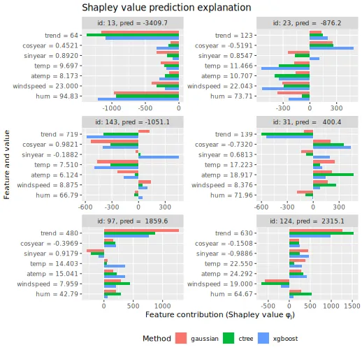

We can also make beeswarm plots of the Shapley values to look at the structure of the Shapley values for all explicands. The figures are quite similar, but with minor differences. E.g., the gaussian approach produces almost no Shapley values around $500$ for the trend feature.

plot_beeswarms(explanation_sym_con, title = "Symmetric conditional Shapley values")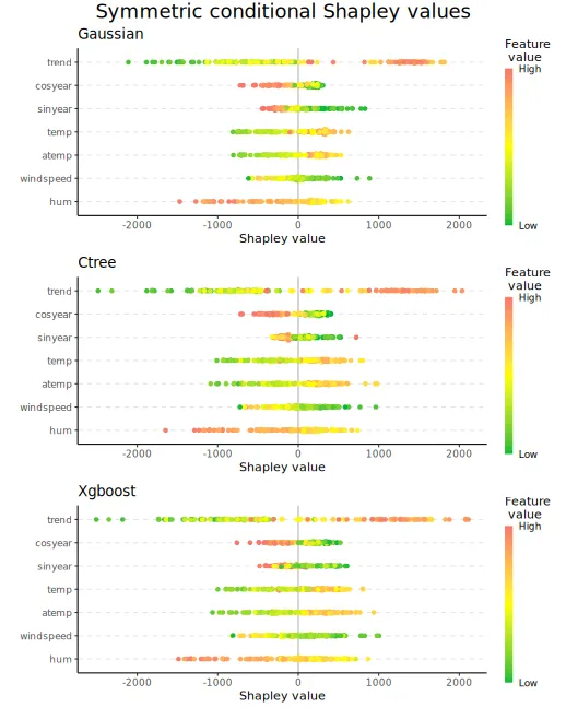

Asymmetric conditional Shapley values

Then we look at the asymmetric conditional Shapley values. To obtain these types of Shapley values, we have to specify that asymmetric = TRUE and a causal_ordering. We use causal_ordering = list(1, c(2, 3), c(4:7)).

explanation_asym_con <- list()

explanation_asym_con[["gaussian"]] <- explain(
  model = model,
  x_train = x_train,
  x_explain = x_explain,
  phi0 = phi0,
  n_MC_samples = 1000,
  approach = "gaussian",
  asymmetric = TRUE,
  causal_ordering = causal_ordering,
  confounding = NULL # Default value
)
#> Note: Feature classes extracted from the model contains NA.
#> Assuming feature classes from the data are correct.
#> Success with message:
#> max_n_coalitions is NULL or larger than or number of coalitions respecting the causal
#> ordering 20, and is therefore set to 20.
#> 
#> ── Starting `shapr::explain()` at 2024-11-21 22:41:52 ──────────────────────────────────────────────────────────────────────────────────────────────────────
#> • Model class: <xgb.Booster>
#> • Approach: gaussian
#> • Iterative estimation: TRUE
#> • Number of feature-wise Shapley values: 7
#> • Number of observations to explain: 144
#> • Number of asymmetric coalitions: 20
#> • Causal ordering: {trend}, {cosyear, sinyear}, {temp, atemp, windspeed, hum}
#> • Computations (temporary) saved at: '/tmp/RtmppO00aE/shapr_obj_1c345f2569ff76.rds'
#> 
#> ── iterative computation started ──
#> 
#> ── Iteration 1 ─────────────────────────────────────────────────────────────────────────────────────────────────────────────────────────────────────────────
#> ℹ Using 13 of 20 coalitions, 13 new.

explanation_asym_con[["gaussian_non_iterative"]] <- explain(
  model = model,
  x_train = x_train,
  x_explain = x_explain,
  phi0 = phi0,
  n_MC_samples = 1000,
  approach = "gaussian",
  asymmetric = TRUE,
  causal_ordering = causal_ordering,
  confounding = NULL, # Default value
  iterative = FALSE
)
#> Note: Feature classes extracted from the model contains NA.
#> Assuming feature classes from the data are correct.
#> Success with message:
#> max_n_coalitions is NULL or larger than or number of coalitions respecting the causal
#> ordering 20, and is therefore set to 20.
#> 
#> ── Starting `shapr::explain()` at 2024-11-21 22:41:54 ──────────────────────────────────────────────────────────────────────────────────────────────────────
#> • Model class: <xgb.Booster>
#> • Approach: gaussian
#> • Iterative estimation: FALSE
#> • Number of feature-wise Shapley values: 7
#> • Number of observations to explain: 144
#> • Number of asymmetric coalitions: 20
#> • Causal ordering: {trend}, {cosyear, sinyear}, {temp, atemp, windspeed, hum}
#> • Computations (temporary) saved at: '/tmp/RtmppO00aE/shapr_obj_1c345f6e6f4e7c.rds'
#> 
#> ── Main computation started ──
#> 
#> ℹ Using 20 of 20 coalitions.

explanation_asym_con[["ctree"]] <- explain(
  model = model,
  x_train = x_train,
  x_explain = x_explain,
  phi0 = phi0,
  n_MC_samples = 1000,
  approach = "ctree",
  asymmetric = TRUE,
  causal_ordering = causal_ordering,
  confounding = NULL # Default value
)
#> Note: Feature classes extracted from the model contains NA.
#> Assuming feature classes from the data are correct.
#> Success with message:
#> max_n_coalitions is NULL or larger than or number of coalitions respecting the causal
#> ordering 20, and is therefore set to 20.
#> 
#> ── Starting `shapr::explain()` at 2024-11-21 22:41:55 ──────────────────────────────────────────────────────────────────────────────────────────────────────
#> • Model class: <xgb.Booster>
#> • Approach: ctree
#> • Iterative estimation: TRUE
#> • Number of feature-wise Shapley values: 7
#> • Number of observations to explain: 144
#> • Number of asymmetric coalitions: 20
#> • Causal ordering: {trend}, {cosyear, sinyear}, {temp, atemp, windspeed, hum}
#> • Computations (temporary) saved at: '/tmp/RtmppO00aE/shapr_obj_1c345f1934da5c.rds'
#> 
#> ── iterative computation started ──
#> 
#> ── Iteration 1 ─────────────────────────────────────────────────────────────────────────────────────────────────────────────────────────────────────────────
#> ℹ Using 13 of 20 coalitions, 13 new.

explanation_asym_con[["xgboost"]] <- explain(
  model = model,
  x_train = x_train,
  x_explain = x_explain,
  phi0 = phi0,
  approach = "regression_separate",
  regression.model = parsnip::boost_tree(engine = "xgboost", mode = "regression"),
  asymmetric = TRUE,
  causal_ordering = causal_ordering,
  confounding = NULL # Default value
)
#> Note: Feature classes extracted from the model contains NA.
#> Assuming feature classes from the data are correct.
#> Success with message:
#> max_n_coalitions is NULL or larger than or number of coalitions respecting the causal
#> ordering 20, and is therefore set to 20.
#> 
#> ── Starting `shapr::explain()` at 2024-11-21 22:42:03 ──────────────────────────────────────────────────────────────────────────────────────────────────────
#> • Model class: <xgb.Booster>
#> • Approach: regression_separate
#> • Iterative estimation: TRUE
#> • Number of feature-wise Shapley values: 7
#> • Number of observations to explain: 144
#> • Number of asymmetric coalitions: 20
#> • Causal ordering: {trend}, {cosyear, sinyear}, {temp, atemp, windspeed, hum}
#> • Computations (temporary) saved at: '/tmp/RtmppO00aE/shapr_obj_1c345f10314ee0.rds'
#> 
#> ── iterative computation started ──
#> 
#> ── Iteration 1 ─────────────────────────────────────────────────────────────────────────────────────────────────────────────────────────────────────────────
#> ℹ Using 13 of 20 coalitions, 13 new.

The asymmetric conditional Shapley value framework is faster as we only consider $20$ coalitions (including empty and grand coalition) instead of all $128$ coalitions (see code below).

print_MSEv_scores_and_time(explanation_asym_con)
#>                            MSEv  MSEv_sd Time (secs)
#> gaussian               330603.3 36828.70        1.56
#> gaussian_non_iterative 306457.7 35411.60        1.32
#> ctree                  260562.1 29428.95        8.31
#> xgboost                307562.1 39362.81        1.50

# Look at the number of coalitions considered. Decreased from 128 to 20.
explanation_sym_con$gaussian$internal$parameters$max_n_coalitions
#> [1] 128
explanation_asym_con$gaussian$internal$parameters$max_n_coalitions
#> [1] 20

# Here we can see the 20 coalitions that respects the causal ordering
explanation_asym_con$gaussian$internal$objects$dt_valid_causal_coalitions[["coalitions"]]
#> [[1]]
#> integer(0)
#> 
#> [[2]]
#> [1] 1
#> 
#> [[3]]
#> [1] 1 2
#> 
#> [[4]]
#> [1] 1 3
#> 
#> [[5]]
#> [1] 1 2 3
#> 
#> [[6]]
#> [1] 1 2 3 4
#> 
#> [[7]]
#> [1] 1 2 3 5
#> 
#> [[8]]
#> [1] 1 2 3 6
#> 
#> [[9]]
#> [1] 1 2 3 7
#> 
#> [[10]]
#> [1] 1 2 3 4 5
#> 
#> [[11]]
#> [1] 1 2 3 4 6
#> 
#> [[12]]
#> [1] 1 2 3 4 7
#> 
#> [[13]]
#> [1] 1 2 3 5 6
#> 
#> [[14]]
#> [1] 1 2 3 5 7
#> 
#> [[15]]
#> [1] 1 2 3 6 7
#> 
#> [[16]]
#> [1] 1 2 3 4 5 6
#> 
#> [[17]]
#> [1] 1 2 3 4 5 7
#> 
#> [[18]]
#> [1] 1 2 3 4 6 7
#> 
#> [[19]]
#> [1] 1 2 3 5 6 7
#> 
#> [[20]]
#> [1] 1 2 3 4 5 6 7

We can then look at the beeswarm plots of the asymmetric conditional Shapley value. The ctree and xgboost approaches produce similar figures, while the gaussian approach both shrinks and groups the Shapley values for the trend feature, while it produces more negative values for the cosyear feature.

When going from symmetric to asymmetric Shapley values, we see that many of the features’ Shapley values are now shrunken closer to zero, especially temp and atemp.

plot_beeswarms(explanation_asym_con, title = "Asymmetric conditional Shapley values")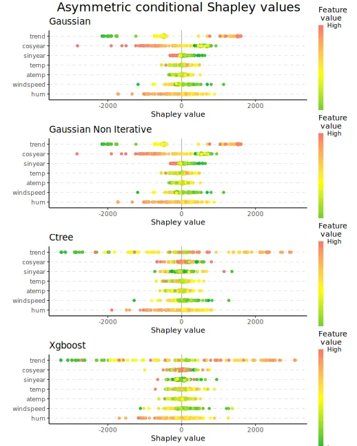

We can also compare the obtained symmetric and asymmetric conditional Shapley values for the 6 explicands. We often see that the asymmetric version gives larger Shapley values to the distal/root causes, i.e., trend and cosyear, than the symmetric version. This is in line with Section 3.2 in Frye, Rowat, and Feige (2020).

# Order the symmetric and asymmetric conditional explanations into a joint list
explanation_sym_con_tmp <- copy(explanation_sym_con)
names(explanation_sym_con_tmp) <- paste0(names(explanation_sym_con_tmp), "_sym")
explanation_asym_con_tmp <- copy(explanation_asym_con)
names(explanation_asym_con_tmp) <- paste0(names(explanation_asym_con_tmp), "_asym")
explanation_asym_sym_con <- c(explanation_sym_con_tmp, explanation_asym_con_tmp)[c(1, 4, 2, 5, 3, 6)]
plot_SV_several_approaches(explanation_asym_sym_con, index_x_explain, brewer_palette = "Paired") +
  theme(legend.position = "bottom")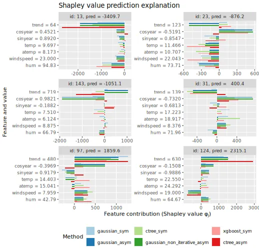

Symmetric marginal Shapley values

For marginal Shapley values, we can only consider the symmetric version as we must set causal_ordering = list(1:7) (or NULL) and confounding = TRUE. Setting asymmetric = TRUE will have no effect, as the causal ordering consists of only a single component containing all features, i.e., all coalitions respect the causal ordering. As stated above, shapr generates the marginal Monte Carlos samples from the Gaussian marginals if approach = "gaussian", while for all other Monte Carlo approaches the marginals are estimated from the training data, i.e., assuming feature independence. Thus, it does not matter if we set approach = "independence" or any other of the Monte Carlo-based approaches. We use approach = "independence" for clarity. Furthermore, we also obtain marginal Shapley values by using the conditional Shapley value framework with the independence approach. However, note that there will be a minuscule difference in the produced Shapley values due to different sampling setups/orders.

explanation_sym_marg <- list()

# Here we sample from the estimated Gaussian marginals
explanation_sym_marg[["gaussian"]] <- explain(
  model = model,
  x_train = x_train,
  x_explain = x_explain,
  phi0 = phi0,
  n_MC_samples = 1000,
  approach = "gaussian",
  asymmetric = FALSE,
  causal_ordering = list(1:7),
  confounding = TRUE
)
#> Note: Feature classes extracted from the model contains NA.
#> Assuming feature classes from the data are correct.
#> Success with message:
#> max_n_coalitions is NULL or larger than or 2^n_features = 128, 
#> and is therefore set to 2^n_features = 128.
#> 
#> ── Starting `shapr::explain()` at 2024-11-21 22:42:07 ──────────────────────────────────────────────────────────────────────────────────────────────────────
#> • Model class: <xgb.Booster>
#> • Approach: gaussian
#> • Iterative estimation: TRUE
#> • Number of feature-wise Shapley values: 7
#> • Number of observations to explain: 144
#> • Causal ordering: {trend, cosyear, sinyear, temp, atemp, windspeed, hum}
#> • Components with confounding: {trend, cosyear, sinyear, temp, atemp, windspeed, hum}
#> • Computations (temporary) saved at: '/tmp/RtmppO00aE/shapr_obj_1c345f39fa59d4.rds'
#> 
#> ── iterative computation started ──
#> 
#> ── Iteration 1 ─────────────────────────────────────────────────────────────────────────────────────────────────────────────────────────────────────────────
#> ℹ Using 13 of 128 coalitions, 13 new.
#> 
#> ── Iteration 2 ─────────────────────────────────────────────────────────────────────────────────────────────────────────────────────────────────────────────
#> ℹ Using 26 of 128 coalitions, 12 new.
#> 
#> ── Iteration 3 ─────────────────────────────────────────────────────────────────────────────────────────────────────────────────────────────────────────────
#> ℹ Using 36 of 128 coalitions, 10 new.

# Here we sample from the marginals of the training data
explanation_sym_marg[["independence_marg"]] <- explain(
  model = model,
  x_train = x_train,
  x_explain = x_explain,
  phi0 = phi0,
  n_MC_samples = 1000,
  approach = "independence",
  asymmetric = FALSE,
  causal_ordering = list(1:7),
  confounding = TRUE
)
#> Note: Feature classes extracted from the model contains NA.
#> Assuming feature classes from the data are correct.
#> Success with message:
#> max_n_coalitions is NULL or larger than or 2^n_features = 128, 
#> and is therefore set to 2^n_features = 128.
#> 
#> ── Starting `shapr::explain()` at 2024-11-21 22:42:17 ──────────────────────────────────────────────────────────────────────────────────────────────────────
#> • Model class: <xgb.Booster>
#> • Approach: independence
#> • Iterative estimation: TRUE
#> • Number of feature-wise Shapley values: 7
#> • Number of observations to explain: 144
#> • Causal ordering: {trend, cosyear, sinyear, temp, atemp, windspeed, hum}
#> • Components with confounding: {trend, cosyear, sinyear, temp, atemp, windspeed, hum}
#> • Computations (temporary) saved at: '/tmp/RtmppO00aE/shapr_obj_1c345f5892ee21.rds'
#> 
#> ── iterative computation started ──
#> 
#> ── Iteration 1 ─────────────────────────────────────────────────────────────────────────────────────────────────────────────────────────────────────────────
#> ℹ Using 13 of 128 coalitions, 13 new.
#> 
#> ── Iteration 2 ─────────────────────────────────────────────────────────────────────────────────────────────────────────────────────────────────────────────
#> ℹ Using 26 of 128 coalitions, 12 new.
#> 
#> ── Iteration 3 ─────────────────────────────────────────────────────────────────────────────────────────────────────────────────────────────────────────────
#> ℹ Using 36 of 128 coalitions, 10 new.

# Here we use the conditional Shapley value framework with the `independence` approach
explanation_sym_marg[["independence_con"]] <- explain(
  model = model,
  x_train = x_train,
  x_explain = x_explain,
  phi0 = phi0,
  n_MC_samples = 1000,
  approach = "independence"
)
#> Note: Feature classes extracted from the model contains NA.
#> Assuming feature classes from the data are correct.
#> Success with message:
#> max_n_coalitions is NULL or larger than or 2^n_features = 128, 
#> and is therefore set to 2^n_features = 128.
#> 
#> ── Starting `shapr::explain()` at 2024-11-21 22:42:30 ──────────────────────────────────────────────────────────────────────────────────────────────────────
#> • Model class: <xgb.Booster>
#> • Approach: independence
#> • Iterative estimation: TRUE
#> • Number of feature-wise Shapley values: 7
#> • Number of observations to explain: 144
#> • Computations (temporary) saved at: '/tmp/RtmppO00aE/shapr_obj_1c345f5be5cbd9.rds'
#> 
#> ── iterative computation started ──
#> 
#> ── Iteration 1 ─────────────────────────────────────────────────────────────────────────────────────────────────────────────────────────────────────────────
#> ℹ Using 13 of 128 coalitions, 13 new.
#> 
#> ── Iteration 2 ─────────────────────────────────────────────────────────────────────────────────────────────────────────────────────────────────────────────
#> ℹ Using 26 of 128 coalitions, 12 new.
#> 
#> ── Iteration 3 ─────────────────────────────────────────────────────────────────────────────────────────────────────────────────────────────────────────────
#> ℹ Using 36 of 128 coalitions, 10 new.

We can look the beeswarm plots

print_MSEv_scores_and_time(explanation_sym_marg)
#>                      MSEv  MSEv_sd Time (secs)
#> gaussian          1383295 111844.8       10.01
#> independence_marg 1382080 111150.6       12.83
#> independence_con  1382544 111313.8       10.01

plot_beeswarms(explanation_sym_marg, title = "Symmetric marginal Shapley values")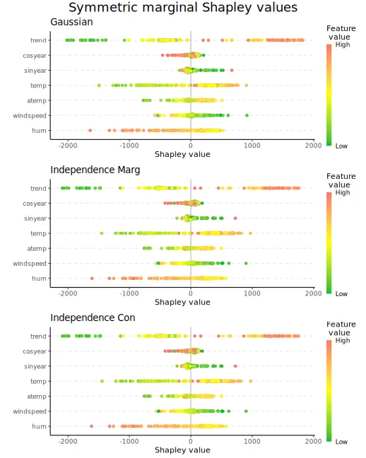

Causal Shapley values

To compute (symmetric/asymmetric) causal Shapley values, we have to provide the causal_ordering and confounding objects. We set them to be causal_ordering = list(1, 2:3, 4:7) and confounding = c(FALSE, TRUE, FALSE), as explained above.

The causal framework takes longer than the other frameworks, as generating the the Monte Carlo samples often consists of a chain of sampling steps. For example, for $\mathcal{S} = {2}$ , we must generate $X_1,X_3,X_4,X_5,X_6,X_7 \mid X_2$ . However, we cannot do this directly due to the causal_ordering and confounding specified above. To generate the Monte Carlo samples, we have to follow a chain of sampling steps. More precisely, we first need to generate $X_1$ from the marginal, then $X_3 \mid X_1$ , and finally $X_4,X_5,X_6,X_7 \mid X_1,X_2,X_3$ . The latter two steps are done by using the provided approach to model the conditional distributions. The internal$objects$S_causal_steps_strings object contains the sampling steps needed for the different feature combinations/coalitions $\mathcal{S}$ .

For causal Shapley values, only the Monte Carlo-based approaches are applicable.

Symmetric

explanation_sym_cau <- list()

explanation_sym_cau[["gaussian"]] <- explain(
  model = model,
  x_train = x_train,
  x_explain = x_explain,
  phi0 = phi0,
  n_MC_samples = 1000,
  approach = "gaussian",
  asymmetric = FALSE,
  causal_ordering = list(1, 2:3, 4:7),
  confounding = c(FALSE, TRUE, FALSE),
  iterative = FALSE, # Set to FALSE to get a single iteration to illustrate sampling steps below
  exact = TRUE
)
#> Note: Feature classes extracted from the model contains NA.
#> Assuming feature classes from the data are correct.
#> Success with message:
#> max_n_coalitions is NULL or larger than or 2^n_features = 128, 
#> and is therefore set to 2^n_features = 128.
#> 
#> ── Starting `shapr::explain()` at 2024-11-21 22:42:41 ──────────────────────────────────────────────────────────────────────────────────────────────────────
#> • Model class: <xgb.Booster>
#> • Approach: gaussian
#> • Iterative estimation: FALSE
#> • Number of feature-wise Shapley values: 7
#> • Number of observations to explain: 144
#> • Causal ordering: {trend}, {cosyear, sinyear}, {temp, atemp, windspeed, hum}
#> • Components with confounding: {cosyear, sinyear}
#> • Computations (temporary) saved at: '/tmp/RtmppO00aE/shapr_obj_1c345f8ccad78.rds'
#> 
#> ── Main computation started ──
#> 
#> ℹ Using 128 of 128 coalitions.

# Look at the sampling steps for the third coalition (S = {2})
explanation_sym_cau$gaussian$internal$iter_list[[1]]$S_causal_steps_strings$id_coalition_3
#> [1] "1|"            "3|1"           "4,5,6,7|1,2,3"

# Use the copula approach
explanation_sym_cau[["copula"]] <- explain(
  model = model,
  x_train = x_train,
  x_explain = x_explain,
  phi0 = phi0,
  n_MC_samples = 1000,
  approach = "copula",
  asymmetric = FALSE,
  causal_ordering = list(1, 2:3, 4:7),
  confounding = c(FALSE, TRUE, FALSE)
)
#> Note: Feature classes extracted from the model contains NA.
#> Assuming feature classes from the data are correct.
#> Success with message:
#> max_n_coalitions is NULL or larger than or 2^n_features = 128, 
#> and is therefore set to 2^n_features = 128.
#> 
#> ── Starting `shapr::explain()` at 2024-11-21 22:43:13 ──────────────────────────────────────────────────────────────────────────────────────────────────────
#> • Model class: <xgb.Booster>
#> • Approach: copula
#> • Iterative estimation: TRUE
#> • Number of feature-wise Shapley values: 7
#> • Number of observations to explain: 144
#> • Causal ordering: {trend}, {cosyear, sinyear}, {temp, atemp, windspeed, hum}
#> • Components with confounding: {cosyear, sinyear}
#> • Computations (temporary) saved at: '/tmp/RtmppO00aE/shapr_obj_1c345f3d6eb8c6.rds'
#> 
#> ── iterative computation started ──
#> 
#> ── Iteration 1 ─────────────────────────────────────────────────────────────────────────────────────────────────────────────────────────────────────────────
#> ℹ Using 13 of 128 coalitions, 13 new.
#> 
#> ── Iteration 2 ─────────────────────────────────────────────────────────────────────────────────────────────────────────────────────────────────────────────
#> ℹ Using 26 of 128 coalitions, 12 new.
#> 
#> ── Iteration 3 ─────────────────────────────────────────────────────────────────────────────────────────────────────────────────────────────────────────────
#> ℹ Using 36 of 128 coalitions, 10 new.

print_MSEv_scores_and_time(explanation_sym_cau)
#>             MSEv  MSEv_sd Time (secs)
#> gaussian 1113795 85800.41       31.94
#> copula   1137608 88376.95       21.69
plot_beeswarms(explanation_sym_cau, title = "Symmetric causal Shapley values")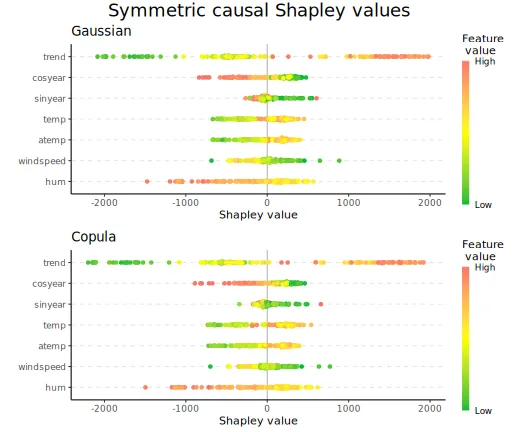

Asymmetric

We now turn to asymmetric causal Shapley values. That is, we only use the coalitions that respects the causal ordering. Thus, the computations are faster as the number of coalitions are reduced.

explanation_asym_cau <- list()

explanation_asym_cau[["gaussian"]] <- explain(
  model = model,
  x_train = x_train,
  x_explain = x_explain,
  phi0 = phi0,
  n_MC_samples = 1000,
  approach = "gaussian",
  asymmetric = TRUE,
  causal_ordering = list(1, 2:3, 4:7),
  confounding = c(FALSE, TRUE, FALSE)
)
#> Note: Feature classes extracted from the model contains NA.
#> Assuming feature classes from the data are correct.
#> Success with message:
#> max_n_coalitions is NULL or larger than or number of coalitions respecting the causal
#> ordering 20, and is therefore set to 20.
#> 
#> ── Starting `shapr::explain()` at 2024-11-21 22:43:36 ──────────────────────────────────────────────────────────────────────────────────────────────────────
#> • Model class: <xgb.Booster>
#> • Approach: gaussian
#> • Iterative estimation: TRUE
#> • Number of feature-wise Shapley values: 7
#> • Number of observations to explain: 144
#> • Number of asymmetric coalitions: 20
#> • Causal ordering: {trend}, {cosyear, sinyear}, {temp, atemp, windspeed, hum}
#> • Components with confounding: {cosyear, sinyear}
#> • Computations (temporary) saved at: '/tmp/RtmppO00aE/shapr_obj_1c345f2b11d871.rds'
#> 
#> ── iterative computation started ──
#> 
#> ── Iteration 1 ─────────────────────────────────────────────────────────────────────────────────────────────────────────────────────────────────────────────
#> ℹ Using 13 of 20 coalitions, 13 new.

# Use the copula approach
explanation_asym_cau[["copula"]] <- explain(
  model = model,
  x_train = x_train,
  x_explain = x_explain,
  phi0 = phi0,
  n_MC_samples = 1000,
  approach = "copula",
  asymmetric = TRUE,
  causal_ordering = list(1, 2:3, 4:7),
  confounding = c(FALSE, TRUE, FALSE)
)
#> Note: Feature classes extracted from the model contains NA.
#> Assuming feature classes from the data are correct.
#> Success with message:
#> max_n_coalitions is NULL or larger than or number of coalitions respecting the causal
#> ordering 20, and is therefore set to 20.
#> 
#> ── Starting `shapr::explain()` at 2024-11-21 22:43:38 ──────────────────────────────────────────────────────────────────────────────────────────────────────
#> • Model class: <xgb.Booster>
#> • Approach: copula
#> • Iterative estimation: TRUE
#> • Number of feature-wise Shapley values: 7
#> • Number of observations to explain: 144
#> • Number of asymmetric coalitions: 20
#> • Causal ordering: {trend}, {cosyear, sinyear}, {temp, atemp, windspeed, hum}
#> • Components with confounding: {cosyear, sinyear}
#> • Computations (temporary) saved at: '/tmp/RtmppO00aE/shapr_obj_1c345f169716e9.rds'
#> 
#> ── iterative computation started ──
#> 
#> ── Iteration 1 ─────────────────────────────────────────────────────────────────────────────────────────────────────────────────────────────────────────────
#> ℹ Using 13 of 20 coalitions, 13 new.
#> 
#> ── Iteration 2 ─────────────────────────────────────────────────────────────────────────────────────────────────────────────────────────────────────────────
#> ℹ Using 14 of 20 coalitions, 1 new.

# Use the vaeac approach
explanation_asym_cau[["vaeac"]] <- explain(
   model = model,
   x_train = x_train,
   x_explain = x_explain,
   phi0 = phi0,
   n_MC_samples = 1000,
   approach = "vaeac",
   vaeac.epochs = 20,
   asymmetric = TRUE,
   causal_ordering = list(1, 2:3, 4:7),
   confounding = c(FALSE, TRUE, FALSE)
 )
#> Note: Feature classes extracted from the model contains NA.
#> Assuming feature classes from the data are correct.
#> Success with message:
#> max_n_coalitions is NULL or larger than or number of coalitions respecting the causal
#> ordering 20, and is therefore set to 20.
#> 
#> ── Starting `shapr::explain()` at 2024-11-21 22:43:42 ──────────────────────────────────────────────────────────────────────────────────────────────────────
#> • Model class: <xgb.Booster>
#> • Approach: vaeac
#> • Iterative estimation: FALSE
#> • Number of feature-wise Shapley values: 7
#> • Number of observations to explain: 144
#> • Number of asymmetric coalitions: 20
#> • Causal ordering: {trend}, {cosyear, sinyear}, {temp, atemp, windspeed, hum}
#> • Components with confounding: {cosyear, sinyear}
#> • Computations (temporary) saved at: '/tmp/RtmppO00aE/shapr_obj_1c345f3b366bf2.rds'
#> 
#> ── Main computation started ──
#> 
#> ℹ Using 20 of 20 coalitions.

We can look at the elapsed time. See the implementation details for an explanation.

print_time(explanation_asym_cau)
#>      gaussian   copula    vaeac
#> [1,] 2.468166 4.216603 451.3722

We can then plot the beeswarm plots.

# Plot the beeswarm plots
plot_beeswarms(explanation_asym_cau, title = "Asymmetric causal Shapley values")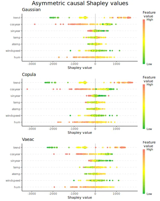

# Plot the Shapley values
plot_SV_several_approaches(explanation_asym_cau, index_x_explain) +
  theme(legend.position = "bottom")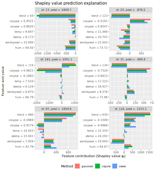

We can also use the other Monte Carlo-based approaches (independence and empirical), too.

Comparing the frameworks

Here we plot the obtained Shapley values for the six explicand when using the gaussian approach in the different Shapley value explanation frameworks, and we see that the different frameworks provide different explanations. The largest difference are between whether we use the symmetric or asymmetric version. To summarize, asymmetric conditional/causal Shapley values focus on the root cause, marginal Shapley values on the more direct effect, and symmetric conditional/causal Shapley consider both for a more natural explanation.

explanation_gaussian <- list(
  symmetric_marginal = explanation_sym_marg$gaussian,
  symmetric_conditional = explanation_sym_con$gaussian,
  symmetric_causal = explanation_sym_cau$gaussian,
  asymmetric_conditional = explanation_asym_con$gaussian,
  asymmetric_causal = explanation_asym_cau$gaussian
)

plot_SV_several_approaches(explanation_gaussian, index_x_explain) +
  theme(legend.position = "bottom") +
  guides(fill = guide_legend(nrow = 2)) +
  ggtitle("Shapley value prediction explanation (approach = 'gaussian')") +
  guides(color = guide_legend(title = "Framework"))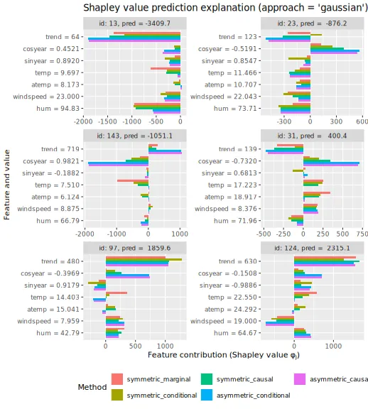

Scatter plots: marginal vs. causal Shapley values

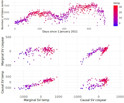
In this section, we produce scatter plots comparing the symmetric marginal and symmetric causal Shapley values for the temperature feature temp and the seasonal feature cosyear for all explicands. The plots shows that the marginal Shapley values almost purely explain the predictions based on temperature, while the causal Shapley values also give credit to season. We can change the features and frameworks in the code below, but we chose these values to replicate Figure 3 in Heskes et al. (2020).

# The color of the points
color <- "temp"

# The features we want to compare
feature_1 <- "cosyear"
feature_2 <- "temp"

# The Shapley value frameworks we want to compare
sv_framework_1 <- explanation_sym_marg[["gaussian"]]
sv_framework_1_str <- "Marginal SV"
sv_framework_2 <- explanation_sym_cau[["gaussian"]]
sv_framework_2_str <- "Causal SV"

# Set up the data.frame we are going to plot
sv_correlation_df <- data.frame(
  color = x_explain[, color],
  sv_framework_1_feature_1 = sv_framework_1$shapley_values_est[[feature_1]],
  sv_framework_2_feature_1 = sv_framework_2$shapley_values_est[[feature_1]],
  sv_framework_1_feature_2 = sv_framework_1$shapley_values_est[[feature_2]],
  sv_framework_2_feature_2 = sv_framework_2$shapley_values_est[[feature_2]]
)

# Make the plots
scatterplot_topleft <-
  ggplot(
    sv_correlation_df,
    aes(x = sv_framework_1_feature_2, y = sv_framework_1_feature_1, color = color)
  ) +
  geom_point(size = 1) +
  xlab(paste(sv_framework_1_str, feature_2)) +
  ylab(paste(sv_framework_1_str, feature_1)) +
  scale_x_continuous(limits = c(-1500, 1000), breaks = c(-1000, 0, 1000)) +
  scale_y_continuous(limits = c(-500, 500), breaks = c(-500, 0, 500)) +
  scale_color_gradient(low = "blue", high = "red") +
  theme_minimal() +
  theme(
    text = element_text(size = 12),
    axis.text.x = element_blank(),
    axis.text.y = element_text(size = 12),
    axis.ticks.x = element_blank(),
    axis.title.x = element_blank()
  )

scatterplot_topright <-
  ggplot(
    sv_correlation_df,
    aes(x = sv_framework_2_feature_1, y = sv_framework_1_feature_1, color = color)
  ) +
  geom_point(size = 1) +
  scale_color_gradient(low = "blue", high = "red") +
  xlab(paste(sv_framework_2_str, feature_1)) +
  ylab(paste(sv_framework_1_str, feature_1)) +
  scale_x_continuous(limits = c(-1500, 1000), breaks = c(-1000, 0, 1000)) +
  scale_y_continuous(limits = c(-500, 500), breaks = c(-500, 0, 500)) +
  theme_minimal() +
  theme(
    text = element_text(size = 12),
    axis.title.x = element_blank(),
    axis.title.y = element_blank(),
    axis.text.x = element_blank(),
    axis.ticks.x = element_blank(),
    axis.text.y = element_blank(),
    axis.ticks.y = element_blank()
  )

scatterplot_bottomleft <-
  ggplot(
    sv_correlation_df,
    aes(x = sv_framework_1_feature_2, y = sv_framework_2_feature_2, color = color)
  ) +
  geom_point(size = 1) +
  scale_color_gradient(low = "blue", high = "red") +
  xlab(paste(sv_framework_1_str, feature_2)) +
  ylab(paste(sv_framework_2_str, feature_2)) +
  scale_x_continuous(limits = c(-1500, 1000), breaks = c(-1000, 0, 1000)) +
  scale_y_continuous(limits = c(-1000, 1000), breaks = c(-500, 0, 500)) +
  theme_minimal() +
  theme(
    text = element_text(size = 12),
    axis.text.x = element_text(size = 12),
    axis.text.y = element_text(size = 12)
  )

scatterplot_bottomright <-
  ggplot(
    sv_correlation_df,
    aes(x = sv_framework_2_feature_1, y = sv_framework_2_feature_2, color = color)
  ) +
  geom_point(size = 1) +
  xlab(paste(sv_framework_2_str, feature_1)) +
  ylab(paste(sv_framework_2_str, feature_2)) +
  scale_x_continuous(limits = c(-1500, 1000), breaks = c(-1000, 0, 1000)) +
  scale_y_continuous(limits = c(-1000, 1000), breaks = c(-500, 0, 500)) +
  scale_color_gradient(low = "blue", high = "red") +
  theme_minimal() +
  theme(
    text = element_text(size = 12),
    axis.text.x = element_text(size = 12),
    axis.title.y = element_blank(),
    axis.text.y = element_blank(),
    axis.ticks.y = element_blank()
  )

# Plot of the trend of the data
bike_plot_new <- ggplot(bike, aes(x = trend, y = cnt, color = get(color))) +
  geom_point(size = 0.75) +
  scale_color_gradient(low = "blue", high = "red") +
  labs(color = color) +
  xlab("Days since 1 January 2011") +
  ylab("Number of bikes rented") +
  theme_minimal() +
  theme(legend.position = "right", legend.title = element_text(size = 10))

# Combine the plots
ggpubr::ggarrange(
  bike_plot_new,
  ggpubr::ggarrange(
    scatterplot_topleft,
    scatterplot_topright,
    scatterplot_bottomleft,
    scatterplot_bottomright,
    legend = "none"
  ),
  nrow = 2, heights = c(1, 2)
)

Investigating two similar days

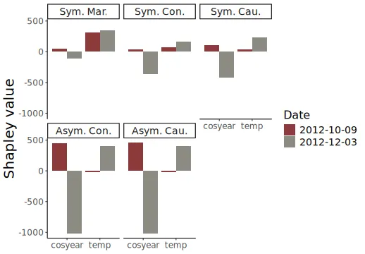
We investigate the difference between symmetric/asymmetric conditional, symmetric/asymmetric causal, and marginal Shapley values for two days: October 10 and December 3, 2012. They have more or less the same temperature of 13 and 13.27 degrees Celsius, and predicted bike counts of 6117 and 6241, respectively. The figure below is an extension of Figure 4 in Heskes et al. (2020), as they only included asymmetric conditional, symmetric causal, and marginal Shapley values.

We plot the various Shapley values for the cosyear and temp features below. We obtain the same results as Heskes et al. (2020) obtained, namely, that the marginal Shapley value explanation framework provides similar explanation for both days. I.e., it only considers the direct effect of temp. The asymmetric conditional and causal Shapley values are almost indistinguishable and put the most weight on the ‘root’ cause cosyear. Heskes et al. (2020) states that the symmetric causal Shapley values provides a sensible balance between the two extremes and gives credit to both season and temperature, but still different explanation for the two days.

However, as we also include symmetric conditional Shapley values, we see that they are extremely similar to symmetric causal Shapley values. I.e., the conditional Shapley value explanation framework also provides a sensible balance between marginal and asymmetric Shapley values. To summarize: as concluded by Heskes et al. (2020) in their Figure 4, the asymmetric conditional/causal Shapley values focus on the root cause, marginal Shapley values on the more direct effect, and symmetric conditional/causal Shapley consider both for a more natural explanation.

# Features of interest
features <- c("cosyear", "temp")

# Get explicands with similar temperature: 2012-10-09 (October) and 2012-12-03 (December)
dates <- c("2012-10-09", "2012-12-03")
dates_idx <- sapply(dates, function(data) which(as.integer(row.names(x_explain)) == which(bike$dteday == data)))
# predict(model, x_explain)[dates_idx] + mean(y_train_nc) # predicted values for the two points

# List of the Shapley value explanations
explanations <- list(
  "Sym. Mar." = explanation_sym_marg[["gaussian"]],
  "Sym. Con." = explanation_sym_con[["gaussian"]],
  "Sym. Cau." = explanation_sym_cau[["gaussian"]],
  "Asym. Con." = explanation_asym_con[["gaussian"]],
  "Asym. Cau." = explanation_asym_cau[["gaussian"]]
)

# Extract the relevant Shapley values
explanations_extracted <- data.table::rbindlist(lapply(seq_along(explanations), function(idx) {
  explanations[[idx]]$shapley_values_est[
    dates_idx, ..features
  ][, `:=`(Date = dates, type = names(explanations)[idx])]
}))

# Set type to be a ordered factor
explanations_extracted[, type := factor(type, levels = names(explanations), ordered = TRUE)]

# Convert from wide to long data table
dt_all <- data.table::melt(explanations_extracted,
  id.vars = c("Date", "type"),
  variable.name = "feature"
)

# Make the plot
ggplot(dt_all, aes(
  x = feature, y = value, group = interaction(Date, feature),
  fill = Date, label = round(value, 2)
)) +
  geom_col(position = "dodge") +
  theme_classic() +
  ylab("Shapley value") +
  facet_wrap(vars(type)) +
  theme(axis.title.x = element_blank()) +
  scale_fill_manual(values = c("indianred4", "ivory4")) +
  theme(
    legend.position.inside = c(0.75, 0.25), axis.title = element_text(size = 20),
    legend.title = element_text(size = 16), legend.text = element_text(size = 14),
    axis.text.x = element_text(size = 12), axis.text.y = element_text(size = 12),
    strip.text.x = element_text(size = 14)
  )

We can also make a similar plot using the plot_SV_several_approaches function in shapr, but then we get each explicand in a separate facet instead of a facet for each framework.

# Here 2012-10-09 is the left facet and 2012-12-03 the right facet
plot_SV_several_approaches(explanations,
  index_explicands = dates_idx,
  only_these_features = features, # Can include more features.
  facet_scales = "free_x",
  horizontal_bars = FALSE,
  axis_labels_n_dodge = 1
) + theme(legend.position = "bottom")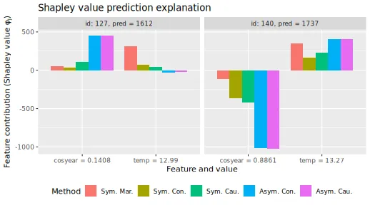

Furthermore, instead of doing as Heskes et al. (2020) and only considering the features cosyear and temp, we can plot all features, too, to get a more complete overview.

# Here 2012-10-09 is the left facet and 2012-12-03 the right facet
plot_SV_several_approaches(explanations,
  index_explicands = dates_idx,
  facet_scales = "free_x",
  horizontal_bars = FALSE,
  axis_labels_rotate_angle = 45,
  digits = 2
) + theme(legend.position = "bottom")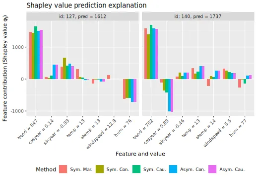

Sampling of coalitions

We can use max_n_coalitions to specify/reduce the number of coalitions to use when computing the Shapley value explanation framework. This applies to marginal, conditional, and causal Shapley values, both the symmetric and asymmetric versions. However, recall that the asymmetric versions already have fewer valid coalitions due to the causal ordering.

In the example below, we demonstrate the sampling of coalitions for the asymmetric and symmetric causal Shapley value explanation frameworks. We half the number of coalitions for both versions and see that the elapsed times are approximately halved, too.

explanation_n_coal <- list()

explanation_n_coal[["sym_cau_gaussian_64"]] <- explain(
  model = model,
  x_train = x_train,
  x_explain = x_explain,
  approach = "gaussian",
  phi0 = phi0,
  asymmetric = FALSE,
  causal_ordering = list(1, 2:3, 4:7),
  confounding = c(FALSE, TRUE, FALSE),
  max_n_coalitions = 64 # Instead of 128
)
#> Note: Feature classes extracted from the model contains NA.
#> Assuming feature classes from the data are correct.
#> 
#> ── Starting `shapr::explain()` at 2024-11-21 22:51:20 ──────────────────────────────────────────────────────────────────────────────────────────────────────
#> • Model class: <xgb.Booster>
#> • Approach: gaussian
#> • Iterative estimation: TRUE
#> • Number of feature-wise Shapley values: 7
#> • Number of observations to explain: 144
#> • Causal ordering: {trend}, {cosyear, sinyear}, {temp, atemp, windspeed, hum}
#> • Components with confounding: {cosyear, sinyear}
#> • Computations (temporary) saved at: '/tmp/RtmppO00aE/shapr_obj_1c345f2da648d9.rds'
#> 
#> ── iterative computation started ──
#> 
#> ── Iteration 1 ─────────────────────────────────────────────────────────────────────────────────────────────────────────────────────────────────────────────
#> ℹ Using 13 of 128 coalitions, 13 new.
#> 
#> ── Iteration 2 ─────────────────────────────────────────────────────────────────────────────────────────────────────────────────────────────────────────────
#> ℹ Using 26 of 128 coalitions, 12 new.
#> 
#> ── Iteration 3 ─────────────────────────────────────────────────────────────────────────────────────────────────────────────────────────────────────────────
#> ℹ Using 36 of 128 coalitions, 10 new.

explanation_n_coal[["asym_cau_gaussian_10"]] <- explain(
  model = model,
  x_train = x_train,
  x_explain = x_explain,
  approach = "gaussian",
  phi0 = phi0,
  asymmetric = TRUE,
  causal_ordering = list(1, 2:3, 4:7),
  confounding = c(FALSE, TRUE, FALSE),
  verbose = c("basic", "convergence", "shapley"),
  max_n_coalitions = 10, # Instead of 20
  iterative = FALSE # Due to small number of coalitions
)
#> Note: Feature classes extracted from the model contains NA.
#> Assuming feature classes from the data are correct.
#> 
#> ── Starting `shapr::explain()` at 2024-11-21 22:51:31 ──────────────────────────────────────────────────────────────────────────────────────────────────────
#> • Model class: <xgb.Booster>
#> • Approach: gaussian
#> • Iterative estimation: FALSE
#> • Number of feature-wise Shapley values: 7
#> • Number of observations to explain: 144
#> • Number of asymmetric coalitions: 20
#> • Causal ordering: {trend}, {cosyear, sinyear}, {temp, atemp, windspeed, hum}
#> • Components with confounding: {cosyear, sinyear}
#> • Computations (temporary) saved at: '/tmp/RtmppO00aE/shapr_obj_1c345f5c86c514.rds'
#> 
#> ── Main computation started ──
#> 
#> ℹ Using 10 of 10 coalitions.
#> 
#> ── Convergence info
#> ✔ Converged after 10 coalitions:
#> Maximum number of iterations reached!
#> Maximum number of coalitions reached!
#> 
#> ── Final estimated Shapley values (sd)
#>              none               trend             cosyear            sinyear               temp              atemp           windspeed                 hum
#>            <char>              <char>              <char>             <char>             <char>             <char>              <char>              <char>
#>   1: 0.00 (0.00)  -2181.910 (374.04)   -825.541 (352.22)  -236.730 (257.69)   -33.813 ( 53.36)    -0.059 ( 65.63)    116.495 ( 58.93)     10.180 ( 92.72) 
#>   2: 0.00 (0.00)  -2174.357 (371.76)   -846.615 (359.93)  -187.083 (274.61)   -44.966 ( 55.88)    34.569 ( 43.16)     13.436 ( 22.08)    185.698 ( 89.51) 
#>   3: 0.00 (0.00)  -2088.959 (360.14)   -793.628 (341.68)  -186.335 (247.79)  -104.809 ( 41.60)   -18.460 ( 53.65)    244.081 ( 54.69)   -122.150 ( 58.72) 
#>   4: 0.00 (0.00)  -2103.364 (368.62)   -798.135 (356.43)  -110.331 (268.86)   169.736 (102.15)    45.240 ( 56.60)   -182.944 ( 57.89)   -207.757 (103.37) 
#>   5: 0.00 (0.00)  -2003.877 (349.11)   -723.936 (323.40)  -231.863 (226.28)    36.505 ( 30.76)     4.713 ( 45.20)    203.889 ( 37.15)    -30.464 ( 60.22) 
#>  ---                                                                                                                                                      
#> 140: 0.00 (0.00)   1575.954 (585.55)  -1014.078 (542.93)   236.336 (357.62)   -68.170 (206.72)    16.388 (172.71)    362.193 (170.75)    627.943 (272.12) 
#> 141: 0.00 (0.00)   1588.686 (607.20)  -1057.223 (537.25)    33.370 (256.33)     1.919 ( 28.74)     7.102 ( 42.27)    216.846 ( 28.79)    -71.698 ( 50.76) 
#> 142: 0.00 (0.00)   1466.745 (593.37)  -1109.151 (522.54)   -96.687 (257.10)   -44.555 ( 72.30)   129.756 ( 53.01)     80.036 ( 24.16)    272.476 (108.15) 
#> 143: 0.00 (0.00)   1003.943 (616.41)  -1780.473 (602.42)  -101.586 (368.10)    19.062 ( 60.65)    -3.841 ( 67.14)     48.680 ( 22.53)   -236.844 ( 96.28) 
#> 144: 0.00 (0.00)    711.139 (724.53)  -2635.898 (777.15)  -178.609 (570.02)    36.623 (147.84)   -66.292 (118.13)   -469.159 ( 81.16)    562.362 (234.12)

# Look at the times
explanation_n_coal[["sym_cau_gaussian_all_128"]] <- explanation_sym_cau$gaussian
explanation_n_coal[["asym_cau_gaussian_all_20"]] <- explanation_asym_cau$gaussian
explanation_n_coal <- explanation_n_coal[c(1, 3, 2, 4)]
print_time(explanation_n_coal)
#>      sym_cau_gaussian_64 sym_cau_gaussian_all_128 asym_cau_gaussian_10 asym_cau_gaussian_all_20
#> [1,]            11.28316                 31.93906             1.905475                 2.468166

We can then plot the beeswarm plots and the Shapley values for the six selected explicands. We see that there are only minuscule differences between the Shapley values we obtain when we use all the coalitions and those we obtain when we use half of the valid coalitions.

plot_beeswarms(explanation_n_coal, title = "Shapley values (gaussian) exact vs. approximation")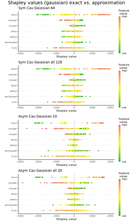

plot_SV_several_approaches(explanation_n_coal, index_x_explain) +
  theme(legend.position = "bottom") +
  guides(fill = guide_legend(nrow = 2))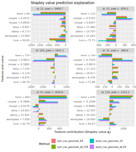

Groups of features

In this section, we demonstrate that we can compute marginal, asymmetric conditional, and symmetric/asymmetric Shapley values for groups of features, too. For group Shapley values, we need to specify the causal ordering on the group level and feature level. We demonstrate with the gaussian approach, but other approaches are applicable, too.

In the pairs plot above (and below), we see that it can be natural to group the features temp and atemp due to their (conceptual) similarity and high correlation.

GGally::ggpairs(x_train[, 4:5])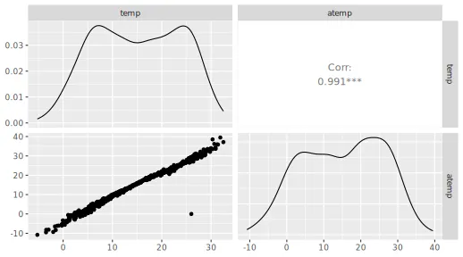

We set up the groups and update the causal ordering to be on the group level.

group_list <- list(
  trend = "trend",
  cosyear = "cosyear",
  sinyear = "sinyear",
  temp_group = c("temp", "atemp"),
  windspeed = "windspeed",
  hum = "hum"
)

causal_ordering_group <-
  list("trend", c("cosyear", "sinyear"), c("temp_group", "windspeed", "hum"))
confounding <- c(FALSE, TRUE, FALSE)

We can then compute the (group) Shapley values using the different Shapley value frameworks.

explanation_group_gaussian <- list()

explanation_group_gaussian[["symmetric_marginal"]] <-
  explain(
    model = model,
    x_train = x_train,
    x_explain = x_explain,
    approach = "gaussian",
    phi0 = phi0,
    asymmetric = FALSE,
    causal_ordering = list(seq(length(group_list))), # or `NULL`
    confounding = TRUE,
    n_MC_samples = 1000,
    group = group_list,
    iterative = FALSE
  )
#> Note: Feature classes extracted from the model contains NA.
#> Assuming feature classes from the data are correct.
#> Success with message:
#> max_n_coalitions is NULL or larger than or 2^n_groups = 64, 
#> and is therefore set to 2^n_groups = 64.
#> 
#> ── Starting `shapr::explain()` at 2024-11-21 22:51:36 ──────────────────────────────────────────────────────────────────────────────────────────────────────
#> • Model class: <xgb.Booster>
#> • Approach: gaussian
#> • Iterative estimation: FALSE
#> • Number of group-wise Shapley values: 6
#> • Number of observations to explain: 144
#> • Causal ordering: {trend, cosyear, sinyear, temp_group, windspeed, hum}
#> • Components with confounding: {trend, cosyear, sinyear, temp_group, windspeed, hum}
#> • Computations (temporary) saved at: '/tmp/RtmppO00aE/shapr_obj_1c345f3eb9f3eb.rds'
#> 
#> ── Main computation started ──
#> 
#> ℹ Using 64 of 64 coalitions.

explanation_group_gaussian[["symmetric_conditional"]] <-
  explain(
    model = model,
    x_train = x_train,
    x_explain = x_explain,
    approach = "gaussian",
    phi0 = phi0,
    asymmetric = FALSE,
    causal_ordering = list(seq(length(group_list))), # or `NULL`
    confounding = NULL,
    n_MC_samples = 1000,
    group = group_list,
    iterative = FALSE
  )
#> Note: Feature classes extracted from the model contains NA.
#> Assuming feature classes from the data are correct.
#> Success with message:
#> max_n_coalitions is NULL or larger than or 2^n_groups = 64, 
#> and is therefore set to 2^n_groups = 64.
#> 
#> ── Starting `shapr::explain()` at 2024-11-21 22:51:46 ──────────────────────────────────────────────────────────────────────────────────────────────────────
#> • Model class: <xgb.Booster>
#> • Approach: gaussian
#> • Iterative estimation: FALSE
#> • Number of group-wise Shapley values: 6
#> • Number of observations to explain: 144
#> • Computations (temporary) saved at: '/tmp/RtmppO00aE/shapr_obj_1c345f3245eb2e.rds'
#> 
#> ── Main computation started ──
#> 
#> ℹ Using 64 of 64 coalitions.

explanation_group_gaussian[["asymmetric_conditional"]] <-
  explain(
    model = model,
    x_train = x_train,
    x_explain = x_explain,
    approach = "gaussian",
    phi0 = phi0,
    asymmetric = TRUE,
    causal_ordering = causal_ordering_group,
    confounding = NULL,
    n_MC_samples = 1000,
    group = group_list,
    iterative = FALSE
  )
#> Note: Feature classes extracted from the model contains NA.
#> Assuming feature classes from the data are correct.
#> Success with message:
#> max_n_coalitions is NULL or larger than or number of coalitions respecting the causal
#> ordering 12, and is therefore set to 12.
#> 
#> ── Starting `shapr::explain()` at 2024-11-21 22:51:51 ──────────────────────────────────────────────────────────────────────────────────────────────────────
#> • Model class: <xgb.Booster>
#> • Approach: gaussian
#> • Iterative estimation: FALSE
#> • Number of group-wise Shapley values: 6
#> • Number of observations to explain: 144
#> • Number of asymmetric coalitions: 12
#> • Causal ordering: {trend}, {cosyear, sinyear}, {temp_group, windspeed, hum}
#> • Computations (temporary) saved at: '/tmp/RtmppO00aE/shapr_obj_1c345f3a65cf0.rds'
#> 
#> ── Main computation started ──
#> 
#> ℹ Using 12 of 12 coalitions.

explanation_group_gaussian[["symmetric_causal"]] <-
  explain(
    model = model,
    x_train = x_train,
    x_explain = x_explain,
    approach = "gaussian",
    phi0 = phi0,
    asymmetric = FALSE,
    causal_ordering = causal_ordering_group,
    confounding = confounding,
    n_MC_samples = 1000,
    group = group_list,
    iterative = FALSE
  )
#> Note: Feature classes extracted from the model contains NA.
#> Assuming feature classes from the data are correct.
#> Success with message:
#> max_n_coalitions is NULL or larger than or 2^n_groups = 64, 
#> and is therefore set to 2^n_groups = 64.
#> 
#> ── Starting `shapr::explain()` at 2024-11-21 22:51:52 ──────────────────────────────────────────────────────────────────────────────────────────────────────
#> • Model class: <xgb.Booster>
#> • Approach: gaussian
#> • Iterative estimation: FALSE
#> • Number of group-wise Shapley values: 6
#> • Number of observations to explain: 144
#> • Causal ordering: {trend}, {cosyear, sinyear}, {temp_group, windspeed, hum}
#> • Components with confounding: {cosyear, sinyear}
#> • Computations (temporary) saved at: '/tmp/RtmppO00aE/shapr_obj_1c345f6ff634f4.rds'
#> 
#> ── Main computation started ──
#> 
#> ℹ Using 64 of 64 coalitions.

explanation_group_gaussian[["asymmetric_causal"]] <-
  explain(
    model = model,
    x_train = x_train,
    x_explain = x_explain,
    approach = "gaussian",
    phi0 = phi0,
    asymmetric = TRUE,
    causal_ordering = causal_ordering_group,
    confounding = confounding,
    n_MC_samples = 1000,
    group = group_list,
    iterative = FALSE
  )
#> Note: Feature classes extracted from the model contains NA.
#> Assuming feature classes from the data are correct.
#> Success with message:
#> max_n_coalitions is NULL or larger than or number of coalitions respecting the causal
#> ordering 12, and is therefore set to 12.
#> 
#> ── Starting `shapr::explain()` at 2024-11-21 22:52:07 ──────────────────────────────────────────────────────────────────────────────────────────────────────
#> • Model class: <xgb.Booster>
#> • Approach: gaussian
#> • Iterative estimation: FALSE
#> • Number of group-wise Shapley values: 6
#> • Number of observations to explain: 144
#> • Number of asymmetric coalitions: 12
#> • Causal ordering: {trend}, {cosyear, sinyear}, {temp_group, windspeed, hum}
#> • Components with confounding: {cosyear, sinyear}
#> • Computations (temporary) saved at: '/tmp/RtmppO00aE/shapr_obj_1c345f32c28e3e.rds'
#> 
#> ── Main computation started ──
#> 
#> ℹ Using 12 of 12 coalitions.

# Look at the elapsed times (symmetric takes the longest time)
print_time(explanation_group_gaussian)
#>      symmetric_marginal symmetric_conditional asymmetric_conditional symmetric_causal asymmetric_causal
#> [1,]           10.38695              4.580573               0.911653         15.69702          1.903805

We can then make the beeswarm plots and Shapley values plots for the six selected explicands. For the beeswarm plots, we set include_group_feature_means = TRUE to make the plots. This means that the plot function use the mean of the temp and atemp features as the feature value. This only makes sense due to the high correlation between the two features.

The main difference between the feature-wise and group-wise Shapley values is that we now see a much wider spread in the Shapley values for temp_group than we did for temp and atemp. For example, for the symmetric causal framework, we saw above that the temp and atemp obtained Shapley values between (around) $-500$ to $500$ , while the grouped version temp_group obtains Shapley values between $-1000$ to $1000$

plot_beeswarms(explanation_group_gaussian,
  title = "Group Shapley values (gaussian)",
  include_group_feature_means = TRUE
)

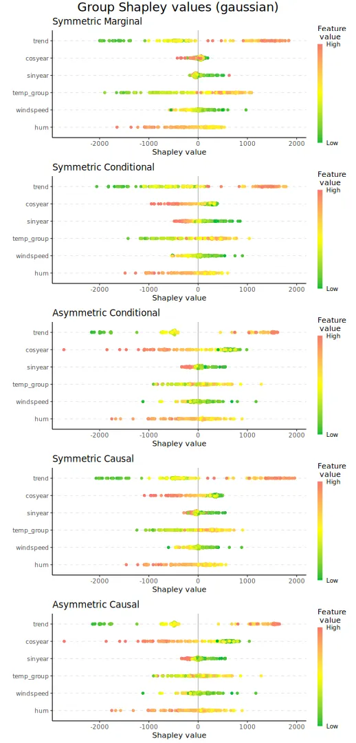
plot_SV_several_approaches(explanation_group_gaussian, index_x_explain) +
  ggtitle("Shapley value prediction explanation (gaussian)") +
  theme(legend.position = "bottom") + guides(fill = guide_legend(nrow = 2))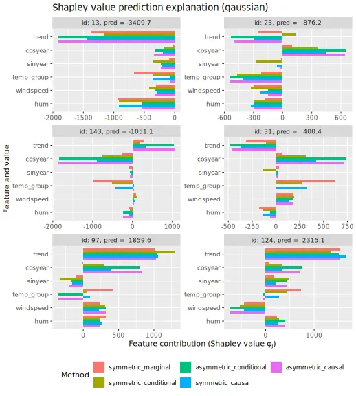

Implementation details

The shapr package is built to estimate conditional Shapley values, thus, it parallelize over the coalitions. This makes perfect sense for said framework as each batch of coalitions are independent of other batches, which means that it is easy to parallelize. Furthermore, by using many batches we drastically reduce the memory usage as shapr does not need to store the Monte Carlo samples for all coalitions.

This setup is not optimal for the causal Shapley value framework as the chains of sampling steps for two coalition $\mathcal{S}$ and $\mathcal{S}^*$ can contain many of the same steps. Ideally, each unique sampling step should only be modeled once to save computation time, but, some of the sampling steps will occur in many of the chains. Thus, we would then have to store the Monte Carlo samples for all coalitions where this sampling step is included, and we can therefor run into memory consumption problems. Thus, in the current implementation, we treat each coalition $\mathcal{S}$ independent and remodel the needed sampling steps for each coalition.

Furthermore, in the conditional Shapley value framework, we have that $\bar{\mathcal{S}} = \mathcal{M} \backslash \mathcal{S}$ , thus shapr will by default generate Monte Carlo samples for all features not in $\mathcal{S}$ . For the causal Shapley value framework, this is not the case, i.e., $\bar{\mathcal{S}} \neq \mathcal{M} \backslash \mathcal{S}$ in general. To reuse the code, we generate Monte Carlo samples for all features not in $\mathcal{S}$ , but only keep the samples for the features in $\bar{\mathcal{S}}$ . To speed up shapr further, one could rewrite all the approaches to support that $\bar{\mathcal{S}}$ is not the complement of $\mathcal{S}$ .

In the code below, we see the unique coalitions/set of features to condition on to generate the Monte Carlo samples for all coalitions and the number of times that set of conditional features is needed in the symmetric causal Shapley value framework for the set up above. We see that most of the conditional distributions will now be remodeled eights times. For the gaussian approach, which is very fast to estimate the conditional distributions, this does not have a major impact on the time. However, for, e.g., the ctree approach which is much slower, this will take a significant amount of extra time. The vaeac approach trains only on these relevant coalitions.

S_causal_steps <- explanation_sym_cau$gaussian$internal$iter_list[[1]]$S_causal_steps
S_causal_unlist <- do.call(c, unlist(S_causal_steps, recursive = FALSE))
S_causal_steps_freq <- S_causal_unlist[grepl("\\.S(?!bar)", names(S_causal_unlist), perl = TRUE)]
S_causal_steps_freq <- S_causal_steps_freq[!sapply(S_causal_steps_freq, is.null)] # Remove NULLs
S_causal_steps_freq <- S_causal_steps_freq[sapply(S_causal_steps_freq, length) > 0] # Remove extra integer(0)
table(sapply(S_causal_steps_freq, paste0, collapse = ","))
#> 
#>           1       1,2,3     1,2,3,4   1,2,3,4,5 1,2,3,4,5,6 1,2,3,4,5,7   1,2,3,4,6 1,2,3,4,6,7   1,2,3,4,7     1,2,3,5   1,2,3,5,6 1,2,3,5,6,7   1,2,3,5,7 
#>          95           7           8           8           8           8           8           8           8           8           8           8           8 
#>     1,2,3,6   1,2,3,6,7     1,2,3,7 
#>           8           8           8

The independence, empirical, ctree, and categorical approaches produce weighted Monte Carlo samples. That means that they do not necessarily generate n_MC_samples. To ensure n_MC_samples, we sample n_MC_samples samples using weighted sampling with replacements where the weights are the weights returned by the approaches.

The marginal Shapley value explanation framework can be extended to support modeling the marginal distributions using the copula and vaeac approaches as both of these methods support unconditional sampling.

References

Aas, Kjersti, Martin Jullum, and Anders Løland. 2021. “Explaining Individual Predictions When Features Are Dependent: More Accurate Approximations to Shapley Values.” Artificial Intelligence 298.

Frye, Christopher, Colin Rowat, and Ilya Feige. 2020. “Asymmetric Shapley Values: Incorporating Causal Knowledge into Model-Agnostic Explainability.” Advances in Neural Information Processing Systems 33: 1229–39.

Heskes, Tom, Evi Sijben, Ioan Gabriel Bucur, and Tom Claassen. 2020. “Causal Shapley Values: Exploiting Causal Knowledge to Explain Individual Predictions of Complex Models.” Advances in Neural Information Processing Systems 33: 4778–89.

Lundberg, Scott M, and Su-In Lee. 2017. “A Unified Approach to Interpreting Model Predictions.” In Advances in Neural Information Processing Systems, 4765–74.

Lars Henry Berge Olsen

Overview

Asymmetric conditional Shapley values

Causal Shapley values

Marginal Shapley values

Symmetric conditioal Shapley values

Code example

Overview

Code setup

Symmetric conditional Shapley values (default)

Asymmetric conditional Shapley values

Symmetric marginal Shapley values

Causal Shapley values

Symmetric

Asymmetric

Comparing the frameworks

Scatter plots: marginal vs. causal Shapley values

Investigating two similar days

Sampling of coalitions

Groups of features

Implementation details

References