Explain the output of machine learning models with dependence-aware (conditional/observational) Shapley values

Compute dependence-aware Shapley values for observations in x_explain from the specified model using the method specified in approach to estimate the conditional expectation. See Aas et al. (2021) for a thorough introduction to dependence-aware prediction explanation with Shapley values. For an overview of the methodology and capabilities of the package, see the software paper Jullum et al. (2025), or the pkgdown site at norskregnesentral.github.io/shapr/.

Usage

explain(
  model,
  x_explain,
  x_train,
  approach,
  phi0,
  iterative = NULL,
  max_n_coalitions = NULL,
  group = NULL,
  n_MC_samples = 1000,
  seed = NULL,
  verbose = "basic",
  predict_model = NULL,
  get_model_specs = NULL,
  prev_shapr_object = NULL,
  asymmetric = FALSE,
  causal_ordering = NULL,
  confounding = NULL,
  extra_computation_args = list(),
  iterative_args = list(),
  output_args = list(),
  ...
)

Arguments

model

Model object. The model whose predictions you want to explain. Run get_supported_models() for a table of which models explain supports natively. Unsupported models can still be explained by passing predict_model and (optionally) get_model_specs, see details for more information.

x_explain

Matrix or data.frame/data.table. Features for which predictions should be explained.

x_train

Matrix or data.frame/data.table. Data used to estimate the (conditional) feature distributions needed to properly estimate the conditional expectations in the Shapley formula.

approach

Character vector of length 1 or one less than the number of features. All elements should either be "gaussian", "copula", "empirical", "ctree", "vaeac", "categorical", "timeseries", "independence", "regression_separate", or "regression_surrogate". The two regression approaches cannot be combined with any other approach. See details for more information.

phi0

Numeric. The prediction value for unseen data, i.e., an estimate of the expected prediction without conditioning on any features. Typically set this equal to the mean of the response in the training data, but alternatives such as the mean of the training predictions are also reasonable.

iterative

Logical or NULL. If NULL (default), set to TRUE if there are more than 5 features/groups, and FALSE otherwise. If TRUE, Shapley values are estimated iteratively for faster, sufficiently accurate results. First an initial number of coalitions is sampled, then bootstrapping estimates the variance of the Shapley values. A convergence criterion determines if the variances are sufficiently small. If not, additional samples are added. The process repeats until the variances are below the threshold. Specifics for the iterative process and convergence criterion are set via iterative_args.

max_n_coalitions

Integer. Upper limit on the number of unique feature/group coalitions to use in the iterative procedure (if iterative = TRUE). If iterative = FALSE, it represents the number of feature/group coalitions to use directly. The quantity refers to the number of unique feature coalitions if group = NULL, and group coalitions if group != NULL. max_n_coalitions = NULL corresponds to 2^n_features.

group

List. If NULL, regular feature-wise Shapley values are computed. If provided, group-wise Shapley values are computed. group then has length equal to the number of groups. Each list element contains the character vectors with the features included in the corresponding group. See Jullum et al. (2021) for more information on group-wise Shapley values.

n_MC_samples

Positive integer. For most approaches, it indicates the maximum number of samples to use in the Monte Carlo integration of every conditional expectation. For approach="ctree", n_MC_samples corresponds to the number of samples from the leaf node (see an exception related to the ctree.sample argument in setup_approach.ctree()). For approach="empirical", n_MC_samples is the \(K\) parameter in equations (14-15) of Aas et al. (2021), i.e. the maximum number of observations (with largest weights) that is used, see also the empirical.eta argument setup_approach.empirical().

seed

Positive integer. Specifies the seed before any code involving randomness is run. If NULL (default), no seed is set in the calling environment.

verbose

String vector or NULL. Controls verbosity (printout detail level) via one or more of "basic", "progress", "convergence", "shapley" and "vS_details". "basic" (default) displays basic information about the computation and messages about parameters/checks. "progress" displays where in the calculation process the function currently is. "convergence" displays how close the Shapley value estimates are to convergence (only when iterative = TRUE). "shapley" displays intermediate Shapley value estimates and standard deviations (only when iterative = TRUE), and the final estimates. "vS_details" displays information about the v(S) estimates, most relevant for approach %in% c("regression_separate", "regression_surrogate", "vaeac"). NULL means no printout. Any combination can be used, e.g., verbose = c("basic", "vS_details").

predict_model

Function. Prediction function to use when model is not natively supported. (Run get_supported_models() for a list of natively supported models.) The function must have two arguments, model and newdata, which specify the model and a data.frame/data.table to compute predictions for, respectively. The function must give the prediction as a numeric vector. NULL (the default) uses functions specified internally. Can also be used to override the default function for natively supported model classes.

get_model_specs

Function. An optional function for checking model/data consistency when model is not natively supported. (Run get_supported_models() for a list of natively supported models.) The function takes model as an argument and provides a list with 3 elements:

labels

Character vector with the names of each feature.

classes

Character vector with the class of each feature.

factor_levels

Character vector with the levels for any categorical features.

If NULL (the default), internal functions are used for natively supported model classes, and checking is disabled for unsupported model classes. Can also be used to override the default function for natively supported model classes.

prev_shapr_object

shapr object or string. If an object of class shapr is provided, or a string with a path to where intermediate results are stored, then the function will use the previous object to continue the computation. This is useful if the computation is interrupted or you want higher accuracy than already obtained, and therefore want to continue the iterative estimation. See the general usage vignette for examples.

asymmetric

Logical. Not applicable for (regular) non-causal explanations. If FALSE (default), explain computes regular symmetric Shapley values. If TRUE, explain computes asymmetric Shapley values based on the (partial) causal ordering given by causal_ordering. That is, explain only uses feature coalitions that respect the causal ordering. If asymmetric is TRUE and confounding is NULL (default), explain computes asymmetric conditional Shapley values as specified in Frye et al. (2020). If confounding is provided, i.e., not NULL, then explain computes asymmetric causal Shapley values as specified in Heskes et al. (2020).

causal_ordering

List. Not applicable for (regular) non-causal or asymmetric explanations. causal_ordering is an unnamed list of vectors specifying the components of the partial causal ordering that the coalitions must respect. Each vector represents a component and contains one or more features/groups identified by their names (strings) or indices (integers). If causal_ordering is NULL (default), no causal ordering is assumed and all possible coalitions are allowed. No causal ordering is equivalent to a causal ordering with a single component that includes all features (list(1:n_features)) or groups (list(1:n_groups)) for feature-wise and group-wise Shapley values, respectively. For feature-wise Shapley values and causal_ordering = list(c(1, 2), c(3, 4)), the interpretation is that features 1 and 2 are the ancestors of features 3 and 4, while features 3 and 4 are on the same level. Note: All features/groups must be included in causal_ordering without duplicates.

confounding

Logical vector. Not applicable for (regular) non-causal or asymmetric explanations. confounding is a logical vector specifying whether confounding is assumed for each component in the causal_ordering. If NULL (default), no assumption about the confounding structure is made and explain computes asymmetric/symmetric conditional Shapley values, depending on asymmetric. If confounding is a single logical (FALSE or TRUE), the assumption is set globally for all components in the causal ordering. Otherwise, confounding must have the same length as causal_ordering, indicating the confounding assumption for each component. When confounding is specified, explain computes asymmetric/symmetric causal Shapley values, depending on asymmetric. The approach cannot be regression_separate or regression_surrogate, as the regression-based approaches are not applicable to the causal Shapley methodology.

extra_computation_args

Named list. Specifies extra arguments related to the computation of the Shapley values. See get_extra_comp_args_default() for description of the arguments and their default values.

iterative_args

Named list. Specifies the arguments for the iterative procedure. See get_iterative_args_default() for description of the arguments and their default values.

output_args

Named list. Specifies certain arguments related to the output of the function. See get_output_args_default() for description of the arguments and their default values.

...

Arguments passed on to setup_approach.categorical, setup_approach.copula, setup_approach.ctree, setup_approach.empirical, setup_approach.gaussian, setup_approach.independence, setup_approach.regression_separate, setup_approach.regression_surrogate, setup_approach.timeseries, setup_approach.vaeac

categorical.joint_prob_dt

Data.table. (Optional) Containing the joint probability distribution for each combination of feature values. NULL means it is estimated from the x_train and x_explain.

categorical.epsilon

Numeric value. (Optional) If categorical.joint_prob_dt is not supplied, probabilities/frequencies are estimated using x_train. If certain observations occur in x_explain and NOT in x_train, then epsilon is used as the proportion of times that these observations occur in the training data. In theory, this proportion should be zero, but this causes an error later in the Shapley computation.

internal

List. Not used directly, but passed through from explain().

ctree.mincriterion

Numeric scalar or vector. Either a scalar or vector of length equal to the number of features in the model. The value is equal to 1 - \(\alpha\) where \(\alpha\) is the nominal level of the conditional independence tests. If it is a vector, this indicates which value to use when conditioning on various numbers of features. The default value is 0.95.

ctree.minsplit

Numeric scalar. Determines the minimum value that the sum of the left and right daughter nodes must reach for a split. The default value is 20.

ctree.minbucket

Numeric scalar. Determines the minimum sum of weights in a terminal node required for a split. The default value is 7.

ctree.sample

Boolean. If TRUE (default), then the method always samples n_MC_samples observations from the leaf nodes (with replacement). If FALSE and the number of observations in the leaf node is less than n_MC_samples, the method will take all observations in the leaf. If FALSE and the number of observations in the leaf node is more than n_MC_samples, the method will sample n_MC_samples observations (with replacement). This means that there will always be sampling in the leaf unless sample = FALSE and the number of obs in the node is less than n_MC_samples.

empirical.type

Character. (default = "fixed_sigma") Must be one of "independence", "fixed_sigma", "AICc_each_k", or "AICc_full". Note: "empirical.type = independence" is deprecated; use approach = "independence" instead. "fixed_sigma" uses a fixed bandwidth (set through empirical.fixed_sigma) in the kernel density estimation. "AICc_each_k" and "AICc_full" optimize the bandwidth using the AICc criterion, with respectively one bandwidth per coalition size and one bandwidth for all coalition sizes.

empirical.eta

Numeric scalar. Needs to be 0 < eta <= 1. The default value is 0.95. Represents the minimum proportion of the total empirical weight that data samples should use. For example, if eta = .8, we choose the K samples with the largest weights so that the sum of the weights accounts for 80\ eta is the \(\eta\) parameter in equation (15) of Aas et al. (2021).

empirical.fixed_sigma

Positive numeric scalar. The default value is 0.1. Represents the kernel bandwidth in the distance computation used when conditioning on all different coalitions. Only used when empirical.type = "fixed_sigma"

empirical.n_samples_aicc

Positive integer. Number of samples to consider in AICc optimization. The default value is 1000. Only used when empirical.type is either "AICc_each_k" or "AICc_full".

empirical.eval_max_aicc

Positive integer. Maximum number of iterations when optimizing the AICc. The default value is 20. Only used when empirical.type is either "AICc_each_k" or "AICc_full".

empirical.start_aicc

Numeric. Start value of the sigma parameter when optimizing the AICc. The default value is 0.1. Only used when empirical.type is either "AICc_each_k" or "AICc_full".

empirical.cov_mat

Numeric matrix. (Optional) The covariance matrix of the data generating distribution used to define the Mahalanobis distance. NULL means it is estimated from x_train.

gaussian.mu

Numeric vector. (Optional) Containing the mean of the data generating distribution. NULL means it is estimated from the x_train.

gaussian.cov_mat

Numeric matrix. (Optional) Containing the covariance matrix of the data generating distribution. NULL means it is estimated from the x_train.

regression.model

A tidymodels object of class model_specs. Default is a linear regression model, i.e., parsnip::linear_reg(). See tidymodels for all possible models, and see the vignette for how to add new/own models. Note, to make it easier to call explain() from Python, the regression.model parameter can also be a string specifying the model which will be parsed and evaluated. For example, "parsnip::rand_forest(mtry = hardhat::tune(), trees = 100, engine = "ranger", mode = "regression")" is also a valid input. It is essential to include the package prefix if the package is not loaded.

regression.tune_values

Either NULL (default), a data.frame/data.table/tibble, or a function. The data.frame must contain the possible hyperparameter value combinations to try. The column names must match the names of the tunable parameters specified in regression.model. If regression.tune_values is a function, then it should take one argument x which is the training data for the current coalition and returns a data.frame/data.table/tibble with the properties described above. Using a function allows the hyperparameter values to change based on the size of the coalition See the regression vignette for several examples. Note, to make it easier to call explain() from Python, the regression.tune_values can also be a string containing an R function. For example, "function(x) return(dials::grid_regular(dials::mtry(c(1, ncol(x)))), levels = 3))" is also a valid input. It is essential to include the package prefix if the package is not loaded.

regression.vfold_cv_para

Either NULL (default) or a named list containing the parameters to be sent to rsample::vfold_cv(). See the regression vignette for several examples.

regression.recipe_func

Either NULL (default) or a function that that takes in a recipes::recipe() object and returns a modified recipes::recipe() with potentially additional recipe steps. See the regression vignette for several examples. Note, to make it easier to call explain() from Python, the regression.recipe_func can also be a string containing an R function. For example, "function(recipe) return(recipes::step_ns(recipe, recipes::all_numeric_predictors(), deg_free = 2))" is also a valid input. It is essential to include the package prefix if the package is not loaded.

regression.surrogate_n_comb

Positive integer. Specifies the number of unique coalitions to apply to each training observation. The default is the number of sampled coalitions in the present iteration. Any integer between 1 and the default is allowed. Larger values requires more memory, but may improve the surrogate model. If the user sets a value lower than the maximum, we sample this amount of unique coalitions separately for each training observations. That is, on average, all coalitions should be equally trained.

timeseries.fixed_sigma

Positive numeric scalar. Represents the kernel bandwidth in the distance computation. The default value is 2.

timeseries.bounds

Numeric vector of length two. Specifies the lower and upper bounds of the timeseries. The default is c(NULL, NULL), i.e. no bounds. If one or both of these bounds are not NULL, we restrict the sampled time series to be between these bounds. This is useful if the underlying time series are scaled between 0 and 1, for example.

vaeac.depth

Positive integer (default is 3). The number of hidden layers in the neural networks of the masked encoder, full encoder, and decoder.

vaeac.width

Positive integer (default is 32). The number of neurons in each hidden layer in the neural networks of the masked encoder, full encoder, and decoder.

vaeac.latent_dim

Positive integer (default is 8). The number of dimensions in the latent space.

vaeac.lr

Positive numeric (default is 0.001). The learning rate used in the torch::optim_adam() optimizer.

vaeac.activation_function

An torch::nn_module() representing an activation function such as, e.g., torch::nn_relu() (default), torch::nn_leaky_relu(), torch::nn_selu(), or torch::nn_sigmoid().

vaeac.n_vaeacs_initialize

Positive integer (default is 4). The number of different vaeac models to initiate in the start. Pick the best performing one after vaeac.extra_parameters$epochs_initiation_phase epochs (default is 2) and continue training that one.

vaeac.epochs

Positive integer (default is 100). The number of epochs to train the final vaeac model. This includes vaeac.extra_parameters$epochs_initiation_phase, where the default is 2.

vaeac.extra_parameters

Named list with extra parameters to the vaeac approach. See vaeac_get_extra_para_default() for description of possible additional parameters and their default values.

Value

Object of class c("shapr", "list"). Contains the following items:

shapley_values_est

data.table with the estimated Shapley values with explained observation in the rows and features along the columns. The column none is the prediction not devoted to any of the features (given by the argument phi0)

shapley_values_sd

data.table with the standard deviation of the Shapley values reflecting the uncertainty in the coalition sampling part of the kernelSHAP procedure. These are, by definition, 0 when all coalitions are used. Only present when extra_computation_args$compute_sd=TRUE, which is the default when iterative = TRUE.

internal

List with the different parameters, data, functions and other output used internally.

pred_explain

Numeric vector with the predictions for the explained observations.

MSEv

List with the values of the MSEv evaluation criterion for the approach. See the MSEv evaluation section in the general usage vignette for details.

timing

List containing timing information for the different parts of the computation. summary contains the time stamps for the start and end time in addition to the total execution time. overall_timing_secs gives the time spent on different parts of the explanation computation. main_computation_timing_secs further decomposes the main computation time into different parts of the computation for each iteration of the iterative estimation routine, if used.

Details

The shapr package implements kernelSHAP estimation of dependence-aware Shapley values with eight different Monte Carlo-based approaches for estimating the conditional distributions of the data. These are all introduced in the general usage vignette. (From R: vignette("general_usage", package = "shapr")). For an overview of the methodology and capabilities of the package, please also see the software paper Jullum et al. (2025). Moreover, Aas et al. (2021) gives a general introduction to dependence-aware Shapley values and the approaches "empirical", "gaussian", "copula", and also discusses "independence". Redelmeier et al. (2020) introduces the approach "ctree". Olsen et al. (2022) introduces the "vaeac" approach. Approach "timeseries" is discussed in Jullum et al. (2021). shapr has also implemented two regression-based approaches "regression_separate" and "regression_surrogate", as described in Olsen et al. (2024). It is also possible to combine the different approaches, see the general usage vignette for more information.

The package also supports the computation of causal and asymmetric Shapley values as introduced by Heskes et al. (2020) and Frye et al. (2020). Asymmetric Shapley values were proposed by Frye et al. (2020) as a way to incorporate causal knowledge in the real world by restricting the possible feature combinations/coalitions when computing the Shapley values to those consistent with a (partial) causal ordering. Causal Shapley values were proposed by Heskes et al. (2020) as a way to explain the total effect of features on the prediction, taking into account their causal relationships, by adapting the sampling procedure in shapr.

The package allows parallelized computation with progress updates through the tightly connected future::future and progressr::progressr packages. See the examples below. For iterative estimation (iterative=TRUE), intermediate results may be printed to the console (according to the verbose argument). Moreover, the intermediate results are written to disk. This combined batch computation of the v(S) values enables fast and accurate estimation of the Shapley values in a memory-friendly manner.

References

• Jullum, M., Olsen, L. H. B., Lachmann, J., & Redelmeier, A. (2025). shapr: Explaining Machine Learning Models with Conditional Shapley Values in R and Python. arXiv preprint arXiv:2504.01842.

• Aas, K., Jullum, M., & Løland, A. (2021). Explaining individual predictions when features are dependent: More accurate approximations to Shapley values. Artificial Intelligence, 298, 103502

• Frye, C., Rowat, C., & Feige, I. (2020). Asymmetric Shapley values: incorporating causal knowledge into model-agnostic explainability. Advances in neural information processing systems, 33, 1229-1239

• Heskes, T., Sijben, E., Bucur, I. G., & Claassen, T. (2020). Causal shapley values: Exploiting causal knowledge to explain individual predictions of complex models. Advances in neural information processing systems, 33, 4778-4789

• Jullum, M., Redelmeier, A. & Aas, K. (2021). Efficient and simple prediction explanations with groupShapley: A practical perspective. Italian Workshop on Explainable Artificial Intelligence 2021.

• Redelmeier, A., Jullum, M., & Aas, K. (2020). Explaining predictive models with mixed features using Shapley values and conditional inference trees. In Machine Learning and Knowledge Extraction: International Cross-Domain Conference, CD-MAKE 2020, Dublin, Ireland, August 25-28, 2020, Proceedings 4 (pp. 117-137). Springer International Publishing.

• Sellereite N., & Jullum, M. (2019). shapr: An R-package for explaining machine learning models with dependence-aware Shapley values. Journal of Open Source Software, 5(46), 2027

• Olsen, L. H., Glad, I. K., Jullum, M., & Aas, K. (2022). Using Shapley values and variational autoencoders to explain predictive models with dependent mixed features. Journal of machine learning research, 23(213), 1-51

• Olsen, L. H. B., Glad, I. K., Jullum, M., & Aas, K. (2024). A comparative study of methods for estimating model-agnostic Shapley value explanations. Data Mining and Knowledge Discovery, 1-48

• Olsen, L. H. B., & Jullum, M. (2024). Improving the Sampling Strategy in KernelSHAP. arXiv e-prints, arXiv-2410

Author

Martin Jullum, Lars Henry Berge Olsen

Examples

# \donttest{

# Load example data
data("airquality")
airquality <- airquality[complete.cases(airquality), ]
x_var <- c("Solar.R", "Wind", "Temp", "Month")
y_var <- "Ozone"

# Split data into test and training data
data_train <- head(airquality, -3)
data_explain <- tail(airquality, 3)

x_train <- data_train[, x_var]
x_explain <- data_explain[, x_var]

# Fit a linear model
lm_formula <- as.formula(paste0(y_var, " ~ ", paste0(x_var, collapse = " + ")))
model <- lm(lm_formula, data = data_train)

# Explain predictions
p <- mean(data_train[, y_var])

# (Optionally) enable parallelization via the future package
if (requireNamespace("future", quietly = TRUE)) {
  future::plan("multisession", workers = 2)
}

# (Optionally) enable progress updates within every iteration via the progressr package
if (requireNamespace("progressr", quietly = TRUE)) {
  progressr::handlers(global = TRUE)
}
#> Error in globalCallingHandlers(condition = global_progression_handler): should not be called with handlers on the stack

# Empirical approach
explain1 <- explain(
  model = model,
  x_explain = x_explain,
  x_train = x_train,
  approach = "empirical",
  phi0 = p,
  n_MC_samples = 1e2
)
#> 
#> ── Starting `shapr::explain()` at 2025-08-27 16:07:59 ──────────────────────────
#> ℹ `max_n_coalitions` is `NULL` or larger than `2^n_features = 16`, and is
#>   therefore set to `2^n_features = 16`.
#> 
#> ── Explanation overview ──
#> 
#> • Model class: <lm>
#> • v(S) estimation class: Monte Carlo integration
#> • Approach: empirical
#> • Procedure: Non-iterative
#> • Number of Monte Carlo integration samples: 100
#> • Number of feature-wise Shapley values: 4
#> • Number of observations to explain: 3
#> • Computations (temporary) saved at: /tmp/RtmpL7N48w/shapr_obj_1cbe7942992.rds
#> 
#> ── Main computation started ──
#> 
#> ℹ Using 16 of 16 coalitions. 

# Gaussian approach
explain2 <- explain(
  model = model,
  x_explain = x_explain,
  x_train = x_train,
  approach = "gaussian",
  phi0 = p,
  n_MC_samples = 1e2
)
#> 
#> ── Starting `shapr::explain()` at 2025-08-27 16:08:01 ──────────────────────────
#> ℹ `max_n_coalitions` is `NULL` or larger than `2^n_features = 16`, and is
#>   therefore set to `2^n_features = 16`.
#> 
#> ── Explanation overview ──
#> 
#> • Model class: <lm>
#> • v(S) estimation class: Monte Carlo integration
#> • Approach: gaussian
#> • Procedure: Non-iterative
#> • Number of Monte Carlo integration samples: 100
#> • Number of feature-wise Shapley values: 4
#> • Number of observations to explain: 3
#> • Computations (temporary) saved at: /tmp/RtmpL7N48w/shapr_obj_1cbe2df0c788.rds
#> 
#> ── Main computation started ──
#> 
#> ℹ Using 16 of 16 coalitions. 

# Gaussian copula approach
explain3 <- explain(
  model = model,
  x_explain = x_explain,
  x_train = x_train,
  approach = "copula",
  phi0 = p,
  n_MC_samples = 1e2
)
#> 
#> ── Starting `shapr::explain()` at 2025-08-27 16:08:02 ──────────────────────────
#> ℹ `max_n_coalitions` is `NULL` or larger than `2^n_features = 16`, and is
#>   therefore set to `2^n_features = 16`.
#> 
#> ── Explanation overview ──
#> 
#> • Model class: <lm>
#> • v(S) estimation class: Monte Carlo integration
#> • Approach: copula
#> • Procedure: Non-iterative
#> • Number of Monte Carlo integration samples: 100
#> • Number of feature-wise Shapley values: 4
#> • Number of observations to explain: 3
#> • Computations (temporary) saved at: /tmp/RtmpL7N48w/shapr_obj_1cbe2f730e45.rds
#> 
#> ── Main computation started ──
#> 
#> ℹ Using 16 of 16 coalitions. 

if (requireNamespace("party", quietly = TRUE)) {
  # ctree approach
  explain4 <- explain(
    model = model,
    x_explain = x_explain,
    x_train = x_train,
    approach = "ctree",
    phi0 = p,
    n_MC_samples = 1e2
  )
}
#> 
#> ── Starting `shapr::explain()` at 2025-08-27 16:08:03 ──────────────────────────
#> ℹ `max_n_coalitions` is `NULL` or larger than `2^n_features = 16`, and is
#>   therefore set to `2^n_features = 16`.
#> 
#> ── Explanation overview ──
#> 
#> • Model class: <lm>
#> • v(S) estimation class: Monte Carlo integration
#> • Approach: ctree
#> • Procedure: Non-iterative
#> • Number of Monte Carlo integration samples: 100
#> • Number of feature-wise Shapley values: 4
#> • Number of observations to explain: 3
#> • Computations (temporary) saved at: /tmp/RtmpL7N48w/shapr_obj_1cbe16380af8.rds
#> 
#> ── Main computation started ──
#> 
#> ℹ Using 16 of 16 coalitions. 

# Combined approach
approach <- c("gaussian", "gaussian", "empirical")
explain5 <- explain(
  model = model,
  x_explain = x_explain,
  x_train = x_train,
  approach = approach,
  phi0 = p,
  n_MC_samples = 1e2
)
#> 
#> ── Starting `shapr::explain()` at 2025-08-27 16:08:05 ──────────────────────────
#> ℹ `max_n_coalitions` is `NULL` or larger than `2^n_features = 16`, and is
#>   therefore set to `2^n_features = 16`.
#> 
#> ── Explanation overview ──
#> 
#> • Model class: <lm>
#> • v(S) estimation class: Monte Carlo integration
#> • Approach: gaussian, gaussian, and empirical
#> • Procedure: Non-iterative
#> • Number of Monte Carlo integration samples: 100
#> • Number of feature-wise Shapley values: 4
#> • Number of observations to explain: 3
#> • Computations (temporary) saved at: /tmp/RtmpL7N48w/shapr_obj_1cbe380c831c.rds
#> 
#> ── Main computation started ──
#> 
#> ℹ Using 16 of 16 coalitions. 

## Printing
print(explain1) # The Shapley values
#>    explain_id  none Solar.R   Wind   Temp Month
#>         <int> <num>   <num>  <num>  <num> <num>
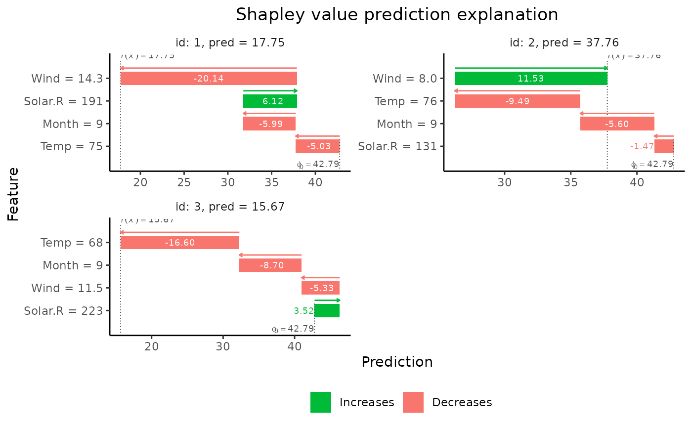
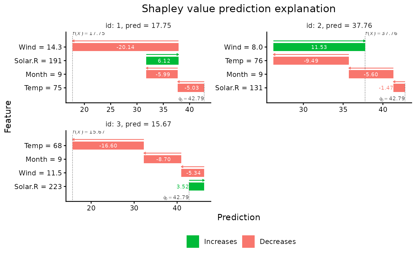
#> 1:          1  42.8    6.12 -20.14  -5.03 -5.99
#> 2:          2  42.8   -1.47  11.53  -9.49 -5.60
#> 3:          3  42.8    3.52  -5.34 -16.60 -8.70
print(explain1) # The Shapley values
#>    explain_id  none Solar.R   Wind   Temp Month
#>         <int> <num>   <num>  <num>  <num> <num>
#> 1:          1  42.8    6.12 -20.14  -5.03 -5.99
#> 2:          2  42.8   -1.47  11.53  -9.49 -5.60
#> 3:          3  42.8    3.52  -5.34 -16.60 -8.70

# The MSEv criterion (+sd). Smaller values indicate a better approach.
print(explain1, what = "MSEv")
#>     MSEv MSEv_sd
#>    <num>   <num>
#> 1:   233    81.6
print(explain2, what = "MSEv")
#>     MSEv MSEv_sd
#>    <num>   <num>
#> 1:   259    90.2
print(explain3, what = "MSEv")
#>     MSEv MSEv_sd
#>    <num>   <num>
#> 1:   224    77.5

## Summary
summary1 <- summary(explain1)
#> 
#> ── Summary of Shapley value explanation ────────────────────────────────────────
#> • Computed with`shapr::explain()` in 2.3 seconds, started 2025-08-27 16:07:59
#> • Model class: <lm>
#> • v(S) estimation class: Monte Carlo integration
#> • Approach: empirical
#> • Procedure: Non-iterative
#> • Number of Monte Carlo integration samples: 100
#> • Number of feature-wise Shapley values: 4
#> • Number of observations to explain: 3
#> • Number of coalitions used: 16 (of total 16)
#> • Computations (temporary) saved at: /tmp/RtmpL7N48w/shapr_obj_1cbe7942992.rds
#> 
#> ── Estimated Shapley values 
#>    explain_id   none Solar.R   Wind   Temp  Month
#>         <int> <char>  <char> <char> <char> <char>
#> 1:          1  42.79    6.12 -20.14  -5.03  -5.99
#> 2:          2  42.79   -1.47  11.53  -9.49  -5.60
#> 3:          3  42.79    3.52  -5.34 -16.60  -8.70
#> 
#> ── Estimated MSEv 
#> Estimated MSE of v(S) = 233 (with sd = 82)

# Various additional info stored in the summary object
# Examples
summary1$shapley_est # A data.table with the Shapley values
#>    explain_id     none   Solar.R       Wind       Temp     Month
#>         <int>    <num>     <num>      <num>      <num>     <num>
#> 1:          1 42.78704  6.124296 -20.137653  -5.033967 -5.987303
#> 2:          2 42.78704 -1.470838  11.525868  -9.487924 -5.597657
#> 3:          3 42.78704  3.524599  -5.335059 -16.599988 -8.703929
summary1$timing$total_time_secs # Total computation time in seconds
#> NULL
summary1$parameters$n_MC_samples # Number of Monte Carlo samples used for the numerical integration
#> [1] 100
summary1$parameters$empirical.type # Type of empirical approach used
#> [1] "fixed_sigma"

# Plot the results
if (requireNamespace("ggplot2", quietly = TRUE)) {
  plot(explain1)
  plot(explain1, plot_type = "waterfall")
}


# Group-wise explanations
group_list <- list(A = c("Temp", "Month"), B = c("Wind", "Solar.R"))

explain_groups <- explain(
  model = model,
  x_explain = x_explain,
  x_train = x_train,
  group = group_list,
  approach = "empirical",
  phi0 = p,
  n_MC_samples = 1e2
)
#> 
#> ── Starting `shapr::explain()` at 2025-08-27 16:08:07 ──────────────────────────
#> ℹ `max_n_coalitions` is `NULL` or larger than `2^n_groups = 4`, and is
#>   therefore set to `2^n_groups = 4`.
#> 
#> ── Explanation overview ──
#> 
#> • Model class: <lm>
#> • v(S) estimation class: Monte Carlo integration
#> • Approach: empirical
#> • Procedure: Non-iterative
#> • Number of Monte Carlo integration samples: 100
#> • Number of group-wise Shapley values: 2
#> • Feature groups: A: {"Temp", "Month"}; B: {"Wind", "Solar.R"}
#> • Number of observations to explain: 3
#> • Computations (temporary) saved at: /tmp/RtmpL7N48w/shapr_obj_1cbecd0dfcb.rds
#> 
#> ── Main computation started ──
#> 
#> ℹ Using 4 of 4 coalitions. 

print(explain_groups)
#>    explain_id  none     A      B
#>         <int> <num> <num>  <num>
#> 1:          1  42.8 -11.6 -13.40
#> 2:          2  42.8 -10.4   5.34
#> 3:          3  42.8 -25.8  -1.32

# Separate and surrogate regression approaches with linear regression models.
req_pkgs <- c("parsnip", "recipes", "workflows", "rsample", "tune", "yardstick")
if (requireNamespace(req_pkgs, quietly = TRUE)) {
  explain_separate_lm <- explain(
    model = model,
    x_explain = x_explain,
    x_train = x_train,
    phi0 = p,
    approach = "regression_separate",
    regression.model = parsnip::linear_reg()
  )

  explain_surrogate_lm <- explain(
    model = model,
    x_explain = x_explain,
    x_train = x_train,
    phi0 = p,
    approach = "regression_surrogate",
    regression.model = parsnip::linear_reg()
  )
}
#> 
#> ── Starting `shapr::explain()` at 2025-08-27 16:08:08 ──────────────────────────
#> ℹ `max_n_coalitions` is `NULL` or larger than `2^n_features = 16`, and is
#>   therefore set to `2^n_features = 16`.
#> 
#> ── Explanation overview ──
#> 
#> • Model class: <lm>
#> • v(S) estimation class: Regression
#> • Approach: regression_separate
#> • Procedure: Non-iterative
#> • Number of feature-wise Shapley values: 4
#> • Number of observations to explain: 3
#> • Computations (temporary) saved at: /tmp/RtmpL7N48w/shapr_obj_1cbe54c49f04.rds
#> 
#> ── Main computation started ──
#> 
#> ℹ Using 16 of 16 coalitions. 
#> 
#> ── Starting `shapr::explain()` at 2025-08-27 16:08:10 ──────────────────────────
#> ℹ `max_n_coalitions` is `NULL` or larger than `2^n_features = 16`, and is
#>   therefore set to `2^n_features = 16`.
#> 
#> ── Explanation overview ──
#> 
#> • Model class: <lm>
#> • v(S) estimation class: Regression
#> • Approach: regression_surrogate
#> • Procedure: Non-iterative
#> • Number of feature-wise Shapley values: 4
#> • Number of observations to explain: 3
#> • Computations (temporary) saved at: /tmp/RtmpL7N48w/shapr_obj_1cbe31b73a3f.rds
#> 
#> ── Main computation started ──
#> 
#> ℹ Using 16 of 16 coalitions. 

# Iterative estimation
# For illustration only. By default not used for such small dimensions as here.
# Restricting the initial and maximum number of coalitions as well.

explain_iterative <- explain(
  model = model,
  x_explain = x_explain,
  x_train = x_train,
  approach = "gaussian",
  phi0 = p,
  iterative = TRUE,
  iterative_args = list(initial_n_coalitions = 8),
  max_n_coalitions = 12
)
#> 
#> ── Starting `shapr::explain()` at 2025-08-27 16:08:11 ──────────────────────────
#> 
#> ── Explanation overview ──
#> 
#> • Model class: <lm>
#> • v(S) estimation class: Monte Carlo integration
#> • Approach: gaussian
#> • Procedure: Iterative
#> • Number of Monte Carlo integration samples: 1000
#> • Number of feature-wise Shapley values: 4
#> • Number of observations to explain: 3
#> • Computations (temporary) saved at: /tmp/RtmpL7N48w/shapr_obj_1cbe35d10ccd.rds
#> 
#> ── Iterative computation started ──
#> 
#> ── Iteration 1 ─────────────────────────────────────────────────────────────────
#> ℹ Using 8 of 16 coalitions, 8 new. 
#> 
#> ── Iteration 2 ─────────────────────────────────────────────────────────────────
#> ℹ Using 10 of 16 coalitions, 2 new. 
#> 
#> ── Iteration 3 ─────────────────────────────────────────────────────────────────
#> ℹ Using 12 of 16 coalitions, 2 new. 

# When not using all coalitions, we can also get the SD of the Shapley values,
# reflecting uncertainty in the coalition sampling part of the procedure.
print(explain_iterative, what = "shapley_sd")
#>    explain_id  none Solar.R  Wind  Temp Month
#>         <int> <num>   <num> <num> <num> <num>
#> 1:          1     0   0.331  1.59  1.74 0.575
#> 2:          2     0   0.367  2.56  2.50 0.696
#> 3:          3     0   0.341  2.94  2.87 0.745

## Summary
# For iterative estimation, convergence info is also provided
summary_iterative <- summary(explain_iterative)
#> 
#> ── Summary of Shapley value explanation ────────────────────────────────────────
#> • Computed with`shapr::explain()` in 4.9 seconds, started 2025-08-27 16:08:11
#> • Model class: <lm>
#> • v(S) estimation class: Monte Carlo integration
#> • Approach: gaussian
#> • Procedure: Iterative
#> • Number of Monte Carlo integration samples: 1000
#> • Number of feature-wise Shapley values: 4
#> • Number of observations to explain: 3
#> • Number of coalitions used: 12 (of total 16)
#> • Computations (temporary) saved at: /tmp/RtmpL7N48w/shapr_obj_1cbe35d10ccd.rds
#> 
#> ── Convergence info 
#> ✔ Iterative Shapley value estimation stopped at 12 coalitions after 3 iterations, due to:
#> Maximum number of coalitions (12) reached!
#> 
#> ── Estimated Shapley values (sd in parentheses) 
#>    explain_id      none      Solar.R          Wind          Temp        Month
#>         <int>    <char>       <char>        <char>        <char>       <char>
#> 1:          1 42.79 (0)  1.83 (0.33) -19.38 (1.59)  -7.12 (1.74) -0.36 (0.57)
#> 2:          2 42.79 (0) -3.49 (0.37)   8.69 (2.56)  -9.56 (2.50) -0.66 (0.70)
#> 3:          3 42.79 (0)  5.15 (0.34)  -4.94 (2.94) -25.98 (2.87) -1.34 (0.75)
#> 
#> ── Estimated MSEv 
#> Estimated MSE of v(S) = 247 (with sd = 101)
# }