shapr: Explaining individual machine learning predictions with Shapley values

Martin Jullum, Camilla Lingjærde, Lars Henry Berge Olsen & Nikolai Sellereite

Introduction

The shapr package implements an extended version of the Kernel SHAP method for approximating Shapley values (Lundberg and Lee (2017)), in which dependence between the features is taken into account (Aas, Jullum, and Løland (2021)).

Estimation of Shapley values is of interest when attempting to explain complex machine learning models. Of existing work on interpreting individual predictions, Shapley values is regarded to be the only model-agnostic explanation method with a solid theoretical foundation (Lundberg and Lee (2017)). Kernel SHAP is a computationally efficient approximation to Shapley values in higher dimensions, but it assumes independent features. Aas, Jullum, and Løland (2021) extends the Kernel SHAP method to handle dependent features, resulting in more accurate approximations to the true Shapley values. See the paper (Aas, Jullum, and Løland (2021)) for further details.

Overview of Package

Functionality

Here is an overview of the main functions. You can read their documentation and see examples with ?function_name.

Main functions in the shapr package.

Function Name	Description
explain	Computes kernel SHAP values for test data.
explain_forecast	Analogous to explain, but for explaining forecasts from time series models.
plot.shapr	Plots the individual prediction explanations. Uses the ggplot and ggbeeswarm package.

The shapr package implements Kernel SHAP estimation of dependence-aware Shapley values with eight different Monte Carlo-based approaches for estimating the conditional distributions of the data, namely "empirical", "gaussian", "copula", "ctree", "vaeac", "categorical", "timeseries", and "independence". shapr has also implemented two regression-based approaches "regression_separate" and "regression_surrogate". See Estimation approaches and plotting functionality below for examples. It is also possible to combine the different approaches, see the combined approach.

The package allows for parallelized computation through the futurepackage, see Parallelization for details.

The level of detail in the output can be controlled through the verbose argument. In addition, progress updates on the process of estimating the v(S)’s (and training the "vaeac" model) is available through the progressr package, supporting progress updates also for parallelized computation. See Verbosity and progress updates for details.

Moreover, the default behavior is to estimate the Shapley values iteratively, with increasing number of feature coalitions being added, and to stop estimation as the estimated Shapley values has achieved a certain level of stability. More information about this is provided in Iterative estimation The above, combined with batch computation of the v(S) values, enables fast and accurate estimation of the Shapley values in a memory friendly manner.

The package also provides functionality for computing Shapley values for groups of features, and custom function explanation, see Advanced usage. Finally, explanation of multiple output time series forecasting models are discussed in Explaining forecasting models.

Default behavior of explain

Below we provide brief descriptions of the most important parts of the default behavior of the explain function.

By default explain always compute feature-wise Shapley values. Groups of features can be explained by providing the feature groups through the group argument.

When there are five or less features (or feature groups), iterative estimation is by default disabled. The reason for this is that it is usually faster to estimate the Shapley values for all possible coalitions (v(S)), than to estimate the uncertainty of the Shapley values, and potentially stop estimation earlier. While iterative estimation is the default starting from six features, it is mainly when there are more than ten features, that it is most beneficial, and can save a lot of computation time. The reason for this is that the number of possible coalitions grows exponentially. These defaults can be overridden by setting the iterative argument to TRUE or FALSE. When using the iterative argument, the estimation for an observation is stopped when all Shapley value standard deviations are below t times the range of the Shapley values. The t value controls the convergence tolerance, defaults to 0.02, and can be set through the iterative_args$convergence_tol argument, see iterative estimation for more details.

Since the iterativeness default changes based on the number of features (or feature groups), the default is also to have no upper bound on the number of coalitions considered. This can be controlled through the max_n_coalitions argument.

Kernel SHAP and dependence-aware estimators

The Kernel SHAP Method

Assume a predictive model $f(\boldsymbol{x})$ for a response value $y$ with features $\boldsymbol{x}\in \mathbb{R}^M$, trained on a training set, and that we want to explain the predictions for new sets of data. This may be done using ideas from cooperative game theory, letting a single prediction take the place of the game being played and the features the place of the players. Letting $N$ denote the set of all $M$ players, and $S \subseteq N$ be a subset of $|S|$ players, the “contribution” function $v(S)$ describes the total expected sum of payoffs the members of $S$ can obtain by cooperation. The Shapley value (Shapley (1953)) is one way to distribute the total gains to the players, assuming that they all collaborate. The amount that player $i$ gets is then

$$\phi_i(v) = \phi_i = \sum_{S \subseteq N \setminus\{i\}} \frac{|S| ! (M-| S| - 1)!}{M!}(v(S\cup \{i\})-v(S)),$$

that is, a weighted mean over all subsets $S$ of players not containing player $i$. Lundberg and Lee (2017) define the contribution function for a certain subset $S$ of these features $\boldsymbol{x}_S$ as $v(S) = \mbox{E}[f(\boldsymbol{x})|\boldsymbol{x}_S]$, the expected output of the predictive model conditional on the feature values of the subset. Lundberg and Lee (2017) names this type of Shapley values SHAP (SHapley Additive exPlanation) values. Since the conditional expectations can be written as

$$\begin{equation} \label{eq:CondExp} E[f(\boldsymbol{x})|\boldsymbol{x}_s=\boldsymbol{x}_S^*] = E[f(\boldsymbol{x}_{\bar{S}},\boldsymbol{x}_S)|\boldsymbol{x}_S=\boldsymbol{x}_S^*] = \int f(\boldsymbol{x}_{\bar{S}},\boldsymbol{x}_S^*)\,p(\boldsymbol{x}_{\bar{S}}|\boldsymbol{x}_S=\boldsymbol{x}_S^*)d\boldsymbol{x}_{\bar{S}}, \end{equation}$$

the conditional distributions $p(\boldsymbol{x}_{\bar{S}}|\boldsymbol{x}_S=\boldsymbol{x}_S^*)$ are needed to compute the contributions. The Kernel SHAP method of Lundberg and Lee (2017) assumes feature independence, so that $p(\boldsymbol{x}_{\bar{S}}|\boldsymbol{x}_S=\boldsymbol{x}_S^*)=p(\boldsymbol{x}_{\bar{S}})$. If samples $\boldsymbol{x}_{\bar{S}}^{k}, k=1,\ldots,K$, from $p(\boldsymbol{x}_{\bar{S}}|\boldsymbol{x}_S=\boldsymbol{x}_S^*)$ are available, the conditional expectation above can be approximated by

$$\begin{equation} v_{\text{KerSHAP}}(S) = \frac{1}{K}\sum_{k=1}^K f(\boldsymbol{x}_{\bar{S}}^{k},\boldsymbol{x}_S^*). \end{equation}$$

In Kernel SHAP, $\boldsymbol{x}_{\bar{S}}^{k}, k=1,\ldots,K$ are sampled from the $\bar{S}$-part of the training data, independently of $\boldsymbol{x}_{S}$. This is motivated by using the training set as the empirical distribution of $\boldsymbol{x}_{\bar{S}}$, and assuming that $\boldsymbol{x}_{\bar{S}}$ is independent of $\boldsymbol{x}_S=\boldsymbol{x}_S^*$. Due to the independence assumption, if the features in a given model are highly dependent, the Kernel SHAP method may give a completely wrong answer. This can be avoided by estimating the conditional distribution $p(\boldsymbol{x}_{\bar{S}}|\boldsymbol{x}_S=\boldsymbol{x}_S^*)$ directly and generating samples from this distribution. With this small change, the contributions and Shapley values may then be approximated as in the ordinary Kernel SHAP framework. Aas, Jullum, and Løland (2021) propose three different approaches for estimating the conditional probabilities which are implemented: empirical, gaussian and copula. The package also implements the ctree method from Redelmeier, Jullum, and Aas (2020), the vaeac method from Olsen et al. (2022) and a categorical for cateogorical data. The original independence approach of Lundberg and Lee (2017) is also available. The methods may also be combined, such that e.g. one method is used when conditioning on a small number of features, while another method is used otherwise. The shapr package also supports directly estimating the contribution function using regression. We briefly introduce the regression-based methods below, but we refer to the separate regression vignette (Shapley value explanations using the regression paradigm) and Olsen et al. (2024) for an in-depth explanation of the regression paradigm.

Multivariate Gaussian Distribution Approach

The first approach arises from the assumption that the feature vector $\boldsymbol{x}$ stems from a multivariate Gaussian distribution with some mean vector $\boldsymbol{\mu}$ and covariance matrix $\boldsymbol{\Sigma}$. Under this assumption, the conditional distribution $p(\boldsymbol{x}_{\bar{\mathcal{S}}} |\boldsymbol{x}_{\mathcal{S}}=\boldsymbol{x}_{\mathcal{S}}^*)$ is also multivariate Gaussian
$\text{N}_{|\bar{\mathcal{S}}|}(\boldsymbol{\mu}_{\bar{\mathcal{S}}|\mathcal{S}},\boldsymbol{\Sigma}_{\bar{\mathcal{S}}|\mathcal{S}})$, with analytical expressions for the conditional mean vector $\boldsymbol{\mu}_{\bar{\mathcal{S}}|\mathcal{S}}$ and covariance matrix $\boldsymbol{\Sigma}_{\bar{\mathcal{S}}|\mathcal{S}}$, see Aas, Jullum, and Løland (2021) for details. Hence, instead of sampling from the marginal empirical distribution of $\boldsymbol{x}_{\bar{\mathcal{S}}}$ approximated by the training data, we can sample from the Gaussian conditional distribution, which is fitted using the training data. Using the resulting samples $\boldsymbol{x}_{\bar{\mathcal{S}}}^k, k=1,\ldots,K$, the conditional expectations be approximated as in the Kernel SHAP.

Gaussian Copula Approach

If the features are far from multivariate Gaussian, an alternative approach is to instead represent the marginals by their empirical distributions, and model the dependence structure by a Gaussian copula. Assuming a Gaussian copula, we may convert the marginals of the training data to Gaussian features using their empirical distributions, and then fit a multivariate Gaussian distribution to these.

To produce samples from the conditional distribution $p(\boldsymbol{x}_{\bar{\mathcal{S}}} |\boldsymbol{x}_{\mathcal{S}}=\boldsymbol{x}_{\mathcal{S}}^*)$, we convert the marginals of $\boldsymbol{x}_{\mathcal{S}}$ to Gaussians, sample from the conditional Gaussian distribution as above, and convert the marginals of the samples back to the original distribution. Those samples are then used to approximate the sample from the resulting multivariate Gaussian conditional distribution. While other copulas may be used, the Gaussian copula has the benefit that we may use the analytical expressions for the conditionals $\boldsymbol{\mu}_{\bar{\mathcal{S}}|\mathcal{S}}$ and $\boldsymbol{\Sigma}_{\bar{\mathcal{S}}|\mathcal{S}}$. Finally, we may convert the marginals back to their original distribution, and use the resulting samples to approximate the conditional expectations as in Kernel SHAP.

Empirical Conditional Distribution Approach

If both the dependence structure and the marginal distributions of $\boldsymbol{x}$ are very far from the Gaussian, neither of the two aforementioned methods will work very well. Few methods exists for the non-parametric estimation of conditional densities, and the classic kernel estimator (Rosenblatt (1956)) for non-parametric density estimation suffers greatly from the curse of dimensionality and does not provide a way to generate samples from the estimated distribution. For such situations, Aas, Jullum, and Løland (2021) propose an empirical conditional approach to sample approximately from $p(\boldsymbol{x}_{\bar{\mathcal{S}}}|\boldsymbol{x}_{\mathcal{S}}^*)$. The idea is to compute weights $w_{\mathcal{S}}(\boldsymbol{x}^*,\boldsymbol{x}^i),\ i=1,...,n_{\text{train}}$ for all training instances based on their Mahalanobis distances (in the $S$ subset only) to the instance $\boldsymbol{x}^*$ to be explained. Instead of sampling from this weighted (conditional) empirical distribution, Aas, Jullum, and Løland (2021) suggests a more efficient variant, using only the $K$ instances with the largest weights:

$$v_{\text{condKerSHAP}}(\mathcal{S}) = \frac{\sum_{k=1}^K w_{\mathcal{S}}(\boldsymbol{x}^*, \boldsymbol{x}^{[k]}) f(\boldsymbol{x}_{\bar{\mathcal{S}}}^{[k]}, \boldsymbol{x}_{\mathcal{S}}^*)}{\sum_{k=1}^K w_{\mathcal{S}}(\boldsymbol{x}^*,\boldsymbol{x}^{[k]})},$$

The number of samples $K$ to be used in the approximate prediction can for instance be chosen such that the $K$ largest weights accounts for a fraction $\eta$, for example $0.9$, of the total weight. If $K$ exceeds a certain limit, for instance $5,000$, it might be set to that limit. A bandwidth parameter $\sigma$ used to scale the weights, must also be specified. This choice may be viewed as a bias-variance trade-off. A small $\sigma$ puts most of the weight to a few of the closest training observations and thereby gives low bias, but high variance. When $\sigma \rightarrow \infty$, this method converges to the original Kernel SHAP assuming feature independence. Typically, when the features are highly dependent, a small $\sigma$ is typically needed such that the bias does not dominate. Aas, Jullum, and Løland (2021) show that a proper criterion for selecting $\sigma$ is a small-sample-size corrected version of the AIC known as AICc. As calculation of it is computationally intensive, an approximate version of the selection criterion is also suggested. Details on this is found in Aas, Jullum, and Løland (2021).

Conditional Inference Tree Approach

The previous three methods can only handle numerical data. This means that if the data contains categorical/discrete/ordinal features, the features first have to be one-hot encoded. When the number of levels/features is large, this is not feasible. An approach that handles mixed (i.e numerical, categorical, discrete, ordinal) features and both univariate and multivariate responses is conditional inference trees (Hothorn, Hornik, and Zeileis (2006)).

Conditional inference trees is a special tree fitting procedure that relies on hypothesis tests to choose both the splitting feature and the splitting point. The tree fitting procedure is sequential: first a splitting feature is chosen (the feature that is least independent of the response), and then a splitting point is chosen for this feature. This decreases the chance of being biased towards features with many splits (Hothorn, Hornik, and Zeileis (2006)).

We use conditional inference trees (ctree) to model the conditional distribution, $p(\boldsymbol{x}_{\bar{\mathcal{S}}}|\boldsymbol{x}_{\mathcal{S}}^*)$, found in the Shapley methodology. First, we fit a different conditional inference tree to each conditional distribution. Once a tree is fit for given dependent features, the end node of $\boldsymbol{x}_{\mathcal{S}}^*$ is found. Then, we sample from this end node and use the resulting samples, $\boldsymbol{x}_{\bar{\mathcal{S}}}^k, k=1,\ldots,K$, when approximating the conditional expectations as in Kernel SHAP. See Redelmeier, Jullum, and Aas (2020) for more details.

The conditional inference trees are fit using the party or partykit packages (Hothorn and Zeileis (2015)).

Variational AutoEncoder with Arbitrary Conditioning (vaeac) Approach

Another approach that supports mixed features is the Variational AutoEncoder with Arbitrary Conditioning (Olsen et al. (2022)), abbreviated to vaeac. The vaeac is an extension of the regular variational autoencoder (Kingma and Welling (2014)), but instead of giving a probabilistic representation of the distribution $p(\boldsymbol{x})$ it gives a probabilistic representation of the conditional distribution $p(\boldsymbol{x}_{\bar{\mathcal{S}}} \mid \boldsymbol{x}_{\mathcal{S}})$, for all possible feature subsets $\mathcal{S}\subseteq\mathcal{M}$ simultaneously, where $\mathcal{M}$ is the set of all features. That is, only a single vaeac model is needed to model all conditional distributions.

The vaeac consists of three neural networks: a full encoder, a masked encoder, and a decoder. The encoders map the full and masked/conditional input representations, i.e., $\boldsymbol{x}$ and $\boldsymbol{x}_{\mathcal{S}}$, respectively, to latent probabilistic representations. Sampled instances from this latent probabilistic representations are sent to the decoder, which maps them back to the feature space and provides a samplable probabilistic representation for the unconditioned features $\boldsymbol{x}_{\bar{\mathcal{S}}}$. The full encoder is only used during the training phase of the vaeac model to guide the training process of the masked encoder, as the former relies on the full input sample $\boldsymbol{x}$, which is not accessible in the deployment phase (when we generate the Monte Carlo samples), as we only have access to $\boldsymbol{x}_{\mathcal{S}}$. The networks are trained by minimizing a variational lower bound. See Section 3 in Olsen et al. (2022) for an in-depth introduction to the vaeac methodology. We use the vaeac model at the epoch which obtains the lowest validation IWAE score to generate the Monte Carlo samples used in the Shapley value computations.

We fit the vaeac model using the R-package torch(Falbel and Luraschi (2023)). The main parameters are the the number of layers in the networks (vaeac.depth), the width of the layers (vaeac.width), the number of dimensions in the latent space (vaeac.latent_dim), the activation function between the layers in the networks (vaeac.activation_function), the learning rate in the ADAM optimizer (vaeac.lr), the number of vaeac models to initiate to remedy poorly initiated model parameter values (vaeac.n_vaeacs_initialize), and the number of learning epochs (vaeac.epochs). See ?shapr::setup_approach.vaeac for a more detailed description of the parameters.

There are additional extra parameters which can be set by including a named list in the call to the explain() function. For example, we can the change the batch size to 32 by including vaeac.extra_parameters = list(vaeac.batch_size = 32) as an argument in the explain() function. See ?shapr::vaeac_get_extra_para_default for a description of the possible extra parameters to the vaeac approach. Note that the main parameters are entered as arguments directly in explain() function, while the extra parameters are specified through a named list called vaeac.extra_parameters.

Categorical Approach

When the features are all categorical, we can estimate the conditional expectations using basic statistical formulas. For example, if we have three features, $x_1, x_2, x_3$ with three levels each (indicated as 1, 2, 3), and we are provided with a table of counts indicating how many times each combination of feature values occurs, we can estimate the marginal and conditional probabilities as follows. Marginal probabilities are estimated by dividing the number of times a given feature (or features) takes on a certain value in the data set with the total number of observations in the data set. Condititional probabilities (for example, $P(X_1 = 1 | X_2 = 1)$) are estimated by first subsetting the data set to reflect the conditioning (i.e., extracting all rows where $X_2 = 1$), and then dividing the number of times the feature on the left hand side of $|$ takes the given value in this subset by the total number of observations in this subset. Once the marginal and conditional probabilities are estimated for all combinations of feature values, each conditional expectation can be calculated. For example, the expected value of $X_1$ given $X_2 = 1$ and $X_3 = 2$ is $$E(X_1|X_2, X_3) = \sum_{x}x P(X_1 = x | X_2=1, X_3=2) = \sum_{x} x \frac{P(X_1 = x, X_2 = 1, X_3 = 2)}{P(X_2=1, X_3=2)}.$$.

Separate and Surrogate Regression Approaches

Another paradigm for estimating the contribution function is the regression paradigm. In contrast to the methods above, which belong to the Monte Carlo paradigm, the regression based methods use regression models to estimate the contribution function $v(S) = E[f(\boldsymbol{x})|\boldsymbol{x}_S = \boldsymbol{x}_S^*]$ directly. The separate regression method class fits a separate regression model for each coalition $S$, while the surrogate regression method class fits a single regression model to simultaneously predict the contribution function for all coalitions. We refer to Olsen et al. (2024) for when one should use the different paradigms, method classes, and methods.

In a separate vignette (Shapley value explanations using the regression paradigm), we elaborate and demonstrate the regression paradigm. We describe how to specify the regression model, enable automatic cross-validation of the model’s hyperparameters, and apply pre-processing steps to the data before fitting the regression models. Olsen et al. (2024) divides the regression paradigm into the separate and surrogate regression method classes. In the separate vignette, we briefly introduce the two method classes. For an in-depth explanation, we refer the reader to Sections 3.5 and 3.6 in Olsen et al. (2024).

Estimation approaches and plotting functionality

The following example shows how a simple xgboost model is trained using the airquality dataset, and how shapr can be used to explain the individual predictions. Since which approach should be used to estimate the contribution functions will depend on the type of data one is working with, the user must specify the approach to be used through the approach argument. Allowed values are "gaussian", "copula", "empirical", "ctree", "vaeac", "categorical", "timeseries", "independence", "regression_separate", and "regression_surrogate".

First we load the shapr package

library(shapr)

library(xgboost)
library(data.table)

data("airquality")
data <- data.table::as.data.table(airquality)
data <- data[complete.cases(data), ]

x_var <- c("Solar.R", "Wind", "Temp", "Month")
y_var <- "Ozone"

ind_x_explain <- 1:6
x_train <- data[-ind_x_explain, ..x_var]
y_train <- data[-ind_x_explain, get(y_var)]
x_explain <- data[ind_x_explain, ..x_var]

# Set seed for reproducibility
set.seed(123)

# Fitting a basic xgboost model to the training data
model <- xgboost::xgboost(
  data = as.matrix(x_train),
  label = y_train,
  nround = 20,
  verbose = FALSE
)

# Specifying the phi_0, i.e. the expected prediction without any features
p0 <- mean(y_train)

# Computing the actual Shapley values with Kernel SHAP accounting for feature dependence using
# the empirical (conditional) distribution approach with bandwidth parameter sigma = 0.1 (default)
explanation <- explain(
  model = model,
  x_explain = x_explain,
  x_train = x_train,
  approach = "empirical",
  phi0 = p0
)
#> Note: Feature classes extracted from the model contains NA.
#> Assuming feature classes from the data are correct.
#> Success with message:
#> max_n_coalitions is NULL or larger than or 2^n_features = 16, 
#> and is therefore set to 2^n_features = 16.
#> 
#> ── Starting `shapr::explain()` at 2024-11-21 20:44:12 ────────────────────────────────────
#> • Model class: <xgb.Booster>
#> • Approach: empirical
#> • Iterative estimation: FALSE
#> • Number of feature-wise Shapley values: 4
#> • Number of observations to explain: 6
#> • Computations (temporary) saved at: '/tmp/RtmpCcS4cy/shapr_obj_1b8c93756774fb.rds'
#> 
#> ── Main computation started ──
#> 
#> ℹ Using 16 of 16 coalitions.

# Printing the Shapley values for the test data.
# For more information about the interpretation of the values in the table, see ?shapr::explain.
print(explanation$shapley_values_est)
#>    explain_id   none  Solar.R    Wind    Temp    Month
#>         <int>  <num>    <num>   <num>   <num>    <num>
#> 1:          1 43.086 13.21173  4.7856 -25.572  -5.5992
#> 2:          2 43.086 -9.97277  5.8307 -11.039  -7.8300
#> 3:          3 43.086 -2.29162 -7.0534 -10.150  -4.4525
#> 4:          4 43.086  3.32546 -3.2409 -10.225  -6.6635
#> 5:          5 43.086  4.30396 -2.6278 -14.152 -12.2669
#> 6:          6 43.086  0.47864 -5.2487 -12.553  -6.6457

# Plot the resulting explanations for observations 1 and 6
plot(explanation, bar_plot_phi0 = FALSE, index_x_explain = c(1, 6))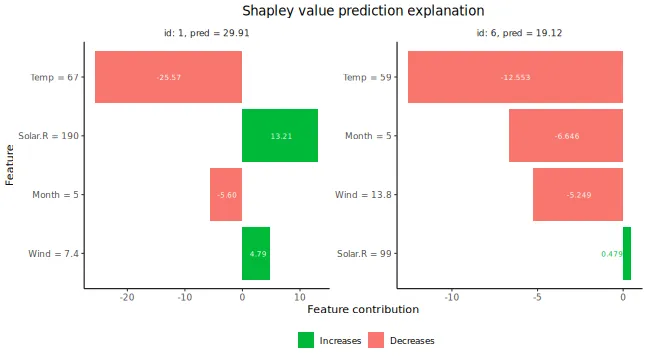

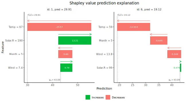
There are multiple plot options specified by the plot_type argument in plot. The waterfall option shows the changes in the prediction score due to each features contribution (their Shapley values):

There are multiple plot options specified by the plot_type argument in plot. The waterfall option shows the changes in the prediction score due to each features contribution (their Shapley values):

plot(explanation, plot_type = "waterfall", index_x_explain = c(1, 6))

The other two plot options, "beeswarm" and "scatter", can be useful when you have many observations that you want to explain. For the purpose of illustration, we explain the whole airquality dataset (including the training data) for these plot types. The plot_type = "beeswarm" summarises the distribution of the Shapley values along the x-axis across all features. Each point gives the Shapley value of a given instance, where the points are colored by the feature value of that instance:

x_explain_many <- data[, ..x_var]
explanation_plot <- explain(
  model = model,
  x_explain = x_explain_many,
  x_train = x_train,
  approach = "empirical",
  phi0 = p0
)
#> Note: Feature classes extracted from the model contains NA.
#> Assuming feature classes from the data are correct.
#> Success with message:
#> max_n_coalitions is NULL or larger than or 2^n_features = 16, 
#> and is therefore set to 2^n_features = 16.
#> 
#> ── Starting `shapr::explain()` at 2024-11-21 20:44:19 ────────────────────────────────────
#> • Model class: <xgb.Booster>
#> • Approach: empirical
#> • Iterative estimation: FALSE
#> • Number of feature-wise Shapley values: 4
#> • Number of observations to explain: 111
#> • Computations (temporary) saved at: '/tmp/RtmpCcS4cy/shapr_obj_1b8c931d8811ab.rds'
#> 
#> ── Main computation started ──
#> 
#> ℹ Using 16 of 16 coalitions.
plot(explanation_plot, plot_type = "beeswarm")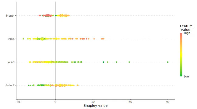

The plot_type = "scatter" plots the feature values on the x-axis and Shapley values on the y-axis, as well as (optionally) a background scatter_hist showing the distribution of the feature data:

plot(explanation_plot, plot_type = "scatter", scatter_hist = TRUE)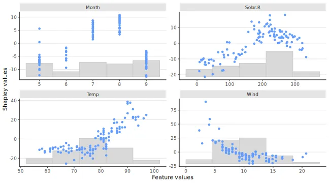

We can use mixed (i.e continuous, categorical, ordinal) data with ctree or vaeac. Use ctree with mixed data in the following manner:

# convert the month variable to a factor
data[, Month_factor := as.factor(Month)]

data_train_cat <- data[-ind_x_explain, ]
data_explain_cat <- data[ind_x_explain, ]

x_var_cat <- c("Solar.R", "Wind", "Temp", "Month_factor")

x_train_cat <- data_train_cat[, ..x_var_cat]
x_explain_cat <- data_explain_cat[, ..x_var_cat]

# Fitting an lm model here as xgboost does not handle categorical features directly
# (work around in example below)
lm_formula <- as.formula(paste0(y_var, " ~ ", paste0(x_var_cat, collapse = " + ")))

model_lm_cat <- lm(lm_formula, data_train_cat)

p0 <- mean(y_train)
explanation_lm_cat <- explain(
  model = model_lm_cat,
  x_explain = x_explain_cat,
  x_train = x_train_cat,
  approach = "ctree",
  phi0 = p0
)
#> Success with message:
#> max_n_coalitions is NULL or larger than or 2^n_features = 16, 
#> and is therefore set to 2^n_features = 16.
#> 
#> ── Starting `shapr::explain()` at 2024-11-21 20:44:31 ────────────────────────────────────
#> • Model class: <lm>
#> • Approach: ctree
#> • Iterative estimation: FALSE
#> • Number of feature-wise Shapley values: 4
#> • Number of observations to explain: 6
#> • Computations (temporary) saved at: '/tmp/RtmpCcS4cy/shapr_obj_1b8c934d11d260.rds'
#> 
#> ── Main computation started ──
#> 
#> ℹ Using 16 of 16 coalitions.

# Plot the resulting explanations for observations 1 and 6, excluding
# the no-covariate effect
plot(explanation_lm_cat, bar_plot_phi0 = FALSE, index_x_explain = c(1, 6))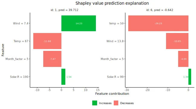

We can specify parameters used to build the conditional inference trees in the following manner. The default values are based on Hothorn, Hornik, and Zeileis (2006).

# Use the conditional inference tree approach
# We can specify parameters used to building trees by specifying mincriterion,
# minsplit, minbucket
explanation_ctree <- explain(
  model = model_lm_cat,
  x_explain = x_explain_cat,
  x_train = x_train_cat,
  approach = "ctree",
  phi0 = p0,
  ctree.mincriterion = 0.80,
  ctree.minsplit = 20,
  ctree.minbucket = 20
)
#> Success with message:
#> max_n_coalitions is NULL or larger than or 2^n_features = 16, 
#> and is therefore set to 2^n_features = 16.
#> 
#> ── Starting `shapr::explain()` at 2024-11-21 20:44:32 ────────────────────────────────────
#> • Model class: <lm>
#> • Approach: ctree
#> • Iterative estimation: FALSE
#> • Number of feature-wise Shapley values: 4
#> • Number of observations to explain: 6
#> • Computations (temporary) saved at: '/tmp/RtmpCcS4cy/shapr_obj_1b8c93a8d4f63.rds'
#> 
#> ── Main computation started ──
#> 
#> ℹ Using 16 of 16 coalitions.
# Default parameters (based on (Hothorn, 2006)) are:
# mincriterion = 0.95
# minsplit = 20
# minbucket = 7

If all features are categorical, one may use the categorical approach as follows:

# For the sake of illustration, convert ALL features to factors
data[, Solar.R_factor := as.factor(cut(Solar.R, 10))]
data[, Wind_factor := as.factor(cut(Wind, 3))]
data[, Temp_factor := as.factor(cut(Temp, 2))]
data[, Month_factor := as.factor(Month)]

data_train_all_cat <- data[-ind_x_explain, ]
data_explain_all_cat <- data[ind_x_explain, ]


x_var_all_cat <- c("Solar.R_factor", "Wind_factor", "Temp_factor", "Month_factor")

x_train_all_cat <- data_train_all_cat[, ..x_var_all_cat]
x_explain_all_cat <- data_explain_all_cat[, ..x_var_all_cat]

# Fit an lm model here
lm_formula_all_cat <- as.formula(paste0(y_var, " ~ ", paste0(x_var_all_cat, collapse = " + ")))

model_lm_all_cat <- lm(lm_formula_all_cat, data_train_all_cat)

explanation_cat_method <- explain(
  model = model_lm_all_cat,
  x_explain = x_explain_all_cat,
  x_train = x_train_all_cat,
  approach = "categorical",
  phi0 = p0
)
#> Success with message:
#> max_n_coalitions is NULL or larger than or 2^n_features = 16, 
#> and is therefore set to 2^n_features = 16.
#> 
#> ── Starting `shapr::explain()` at 2024-11-21 20:44:33 ────────────────────────────────────
#> • Model class: <lm>
#> • Approach: categorical
#> • Iterative estimation: FALSE
#> • Number of feature-wise Shapley values: 4
#> • Number of observations to explain: 6
#> • Computations (temporary) saved at: '/tmp/RtmpCcS4cy/shapr_obj_1b8c9361d2d6a5.rds'
#> 
#> ── Main computation started ──
#> 
#> ℹ Using 16 of 16 coalitions.

Shapley values can be used to explain any predictive model. For predictive models taking time series as input, approach='timeseries' can be used. In such models, joint behavior of consecutive time points is often more important for the outcome than the single time points. Therefore, it makes sense to derive Shapley value segments of the time series instead of for each single time point. In shapr this can be achieved through the group attribute. Other optional parameters of approach='timeseries' are timeseries.fixed_sigma and timeseries.bounds (a vector indicating upper and lower bounds of the time series if necessary).

# Simulate time series data with AR(1)-structure
set.seed(1)
data_ts <- data.frame(matrix(NA, ncol = 41, nrow = 4))
for (n in 1:100) {
  set.seed(n)
  e <- rnorm(42, mean = 0, sd = 1)

  m_1 <- 0
  for (i in 2:length(e)) {
    m_1[i] <- 1 + 0.8 * m_1[i - 1] + e[i]
  }
  data_ts[n, ] <- m_1[-1]
}
data_ts <- data.table::as.data.table(data_ts)

x_var_ts <- paste0("X", 1:40)
y_var_ts <- "X41"

ind_x_explain <- 1:6
data_ts_train <- data_ts[-ind_x_explain]

# Creating a predictive model (for illustration just predicting the next point in the time series with a linear model)
lm_ts_formula <- as.formula(X41 ~ .)
model_lm_ts <- lm(lm_ts_formula, data_ts_train)

x_explain_ts <- data_ts[ind_x_explain, ..x_var_ts]
x_train_ts <- data_ts[-ind_x_explain, ..x_var_ts]

# Spitting the time series into 4 segments
group_ts <- list(
  S1 = paste0("X", 1:10),
  S2 = paste0("X", 11:20),
  S3 = paste0("X", 21:30),
  S4 = paste0("X", 31:40)
)


p0_ts <- mean(unlist(data_ts_train[, ..y_var_ts]))

explanation_timeseries <- explain(
  model = model_lm_ts,
  x_explain = x_explain_ts,
  x_train = x_train_ts,
  approach = "timeseries",
  phi0 = p0_ts,
  group = group_ts
)
#> Success with message:
#> max_n_coalitions is NULL or larger than or 2^n_groups = 16, 
#> and is therefore set to 2^n_groups = 16.
#> 
#> ── Starting `shapr::explain()` at 2024-11-21 20:44:33 ────────────────────────────────────
#> • Model class: <lm>
#> • Approach: timeseries
#> • Iterative estimation: FALSE
#> • Number of group-wise Shapley values: 4
#> • Number of observations to explain: 6
#> • Computations (temporary) saved at: '/tmp/RtmpCcS4cy/shapr_obj_1b8c933989300e.rds'
#> 
#> ── Main computation started ──
#> 
#> ℹ Using 16 of 16 coalitions.

MSEv evaluation criterion

We can use the $\operatorname{MSE}_{v}$ criterion proposed by Frye et al. (2021), and later used by, e.g., Olsen et al. (2022) and Olsen et al. (2024), to evaluate and rank the approaches/methods. The $\operatorname{MSE}_{v}$ is given by

$$\begin{align} \label{eq:MSE_v} \operatorname{MSE}_{v} = \operatorname{MSE}_{v}(\text{method } \texttt{q}) = \frac{1}{N_\mathcal{S}} \sum_{\mathcal{S} \in \mathcal{P}^*(\mathcal{M})} \frac{1}{N_\text{explain}} \sum_{i=1}^{N_\text{explain}} \left( f(\boldsymbol{x}^{[i]}) - {\hat{v}}_{\texttt{q}}(\mathcal{S}, \boldsymbol{x}^{[i]})\right)^2\!, \end{align}$$

where ${\hat{v}}_{\texttt{q}}$ is the estimated contribution function using method $\texttt{q}$ and $N_\mathcal{S} = |\mathcal{P}^*(\mathcal{M})| = 2^M-2$, i.e., we have removed the empty ($\mathcal{S} = \emptyset$) and the grand combinations ($\mathcal{S} = \mathcal{M}$) as they are method independent. Meaning that these two combinations do not influence the ranking of the methods as the methods are not used to compute the contribution function for them.

The motivation behind the $\operatorname{MSE}_{v}$ criterion is that $\mathbb{E}_\mathcal{S}\mathbb{E}_{\boldsymbol{x}} (v_{\texttt{true}}(\mathcal{S},\boldsymbol{x}) - \hat{v}_{\texttt{q}}(\mathcal{S}, \boldsymbol{x}))^2$ can be decomposed as

$$\begin{align} \label{eq:expectation_decomposition} \begin{split} \mathbb{E}_\mathcal{S}\mathbb{E}_{\boldsymbol{x}} (v_{\texttt{true}}(\mathcal{S}, \boldsymbol{x})- \hat{v}_{\texttt{q}}(\mathcal{S}, \boldsymbol{x}))^2 &= \mathbb{E}_\mathcal{S}\mathbb{E}_{\boldsymbol{x}} (f(\boldsymbol{x}) - \hat{v}_{\texttt{q}}(\mathcal{S}, \boldsymbol{x}))^2 \\ &\phantom{\,\,\,\,\,\,\,}- \mathbb{E}_\mathcal{S}\mathbb{E}_{\boldsymbol{x}} (f(\boldsymbol{x})-v_{\texttt{true}}(\mathcal{S}, \boldsymbol{x}))^2, \end{split} \end{align}$$

see Appendix A in Covert, Lundberg, and Lee (2020). The first term on the right-hand side of the equation above can be estimated by $\operatorname{MSE}_{v}$, while the second term is a fixed (unknown) constant not influenced by the approach . Thus, a low value of $\operatorname{MSE}_{v}$ indicates that the estimated contribution function $\hat{v}_{\texttt{q}}$ is closer to the true counterpart $v_{\texttt{true}}$ than a high value.

In shapr, we allow for weighting the combinations in the $\operatorname{MSE}_{v}$ evaluation criterion either uniformly or by using the corresponding Shapley kernel weights (or the sampling frequencies when sampling of combinations is used). This is determined by the logical parameter MSEv_uniform_comb_weights in the explain() function, and the default is to do uniform weighting, that is, MSEv_uniform_comb_weights = TRUE.

Advantage:

An advantage of the $\operatorname{MSE}_{v}$ criterion is that $v_\texttt{true}$ is not involved. Thus, we can apply it as an evaluation criterion to real-world data sets where the true Shapley values are unknown.

Disadvantages:

First, we can only use the $\operatorname{MSE}_{v}$ criterion to rank the methods and not assess their closeness to the optimum since the minimum value of the $\operatorname{MSE}_{v}$ criterion is unknown. Second, the criterion evaluates the contribution functions and not the Shapley values.

Olsen et al. (2024) observed a relatively linear relationship between the $\operatorname{MSE}_{v}$ criterion and the mean absolute error $(\operatorname{MAE})$ between the true and estimated Shapley values in extensive simulation studies where the true Shapley values were known. That is, a method that achieves a low $\operatorname{MSE}_{v}$ score also tends to obtain a low $\operatorname{MAE}$ score, and vice versa.

Confidence intervals

The $\operatorname{MSE}_{v}$ criterion can be written as $\operatorname{MSE}_{v} = \frac{1}{N_\text{explain}}\sum_{i=1}^{N_\text{explain}} \operatorname{MSE}_{v,\text{explain }i}$. We can therefore use the central limit theorem to compute an approximate confidence interval for the $\operatorname{MSE}_{v}$ criterion. We have that $\operatorname{MSE}_{v} \pm t_{\alpha/2}\frac{\operatorname{SD}(\operatorname{MSE}_{v})}{\sqrt{N_\text{explain}}}$ is a $(1-\alpha/2)\%$ approximate confidence interval for the evaluation criterion, where $t_{\alpha/2}$ is the $\alpha/2$ percentile of the $T_{N_\text{explain}-1}$ distribution. Note that $N_\text{explain}$ should be large (rule of thumb is at least $30$) for the central limit theorem to be valid. The quantities $\operatorname{MSE}_{v}$ and $\frac{\operatorname{SD}(\operatorname{MSE}_{v})}{\sqrt{N_\text{explain}}}$ are returned by the explain() function in the MSEv list of data tables. We can also compute similar approximate confidence interval for $\operatorname{MSE}_{v}$ criterion for each combination/coalition when only averaging over the observations. However, it does not make sense in the other direction, i.e., when only averaging over the combinations for each observation, as each combination is a different prediction tasks.

MSEv examples

Start by explaining the predictions by using different methods and combining them into lists.

# We use more explicands here for more stable confidence intervals
ind_x_explain_many <- 1:25
x_train <- data[-ind_x_explain_many, ..x_var]
y_train <- data[-ind_x_explain_many, get(y_var)]
x_explain <- data[ind_x_explain_many, ..x_var]

# Fitting a basic xgboost model to the training data
model <- xgboost::xgboost(
  data = as.matrix(x_train),
  label = y_train,
  nround = 20,
  verbose = FALSE
)

# Specifying the phi_0, i.e. the expected prediction without any features
p0 <- mean(y_train)

# Independence approach
explanation_independence <- explain(
  model = model,
  x_explain = x_explain,
  x_train = x_train,
  approach = "independence",
  phi0 = p0,
  n_MC_samples = 1e2,
  MSEv_uniform_comb_weights = TRUE
)
#> Note: Feature classes extracted from the model contains NA.
#> Assuming feature classes from the data are correct.
#> Success with message:
#> max_n_coalitions is NULL or larger than or 2^n_features = 16, 
#> and is therefore set to 2^n_features = 16.
#> 
#> ── Starting `shapr::explain()` at 2024-11-21 20:44:35 ────────────────────────────────────
#> • Model class: <xgb.Booster>
#> • Approach: independence
#> • Iterative estimation: FALSE
#> • Number of feature-wise Shapley values: 4
#> • Number of observations to explain: 25
#> • Computations (temporary) saved at: '/tmp/RtmpCcS4cy/shapr_obj_1b8c9321f2ff20.rds'
#> 
#> ── Main computation started ──
#> 
#> ℹ Using 16 of 16 coalitions.

# Empirical approach
explanation_empirical <- explain(
  model = model,
  x_explain = x_explain,
  x_train = x_train,
  approach = "empirical",
  phi0 = p0,
  n_MC_samples = 1e2,
  MSEv_uniform_comb_weights = TRUE
)
#> Note: Feature classes extracted from the model contains NA.
#> Assuming feature classes from the data are correct.
#> Success with message:
#> max_n_coalitions is NULL or larger than or 2^n_features = 16, 
#> and is therefore set to 2^n_features = 16.
#> 
#> ── Starting `shapr::explain()` at 2024-11-21 20:44:36 ────────────────────────────────────
#> • Model class: <xgb.Booster>
#> • Approach: empirical
#> • Iterative estimation: FALSE
#> • Number of feature-wise Shapley values: 4
#> • Number of observations to explain: 25
#> • Computations (temporary) saved at: '/tmp/RtmpCcS4cy/shapr_obj_1b8c9372002e18.rds'
#> 
#> ── Main computation started ──
#> 
#> ℹ Using 16 of 16 coalitions.

# Gaussian 1e1 approach
explanation_gaussian_1e1 <- explain(
  model = model,
  x_explain = x_explain,
  x_train = x_train,
  approach = "gaussian",
  phi0 = p0,
  n_MC_samples = 1e1,
  MSEv_uniform_comb_weights = TRUE
)
#> Note: Feature classes extracted from the model contains NA.
#> Assuming feature classes from the data are correct.
#> Success with message:
#> max_n_coalitions is NULL or larger than or 2^n_features = 16, 
#> and is therefore set to 2^n_features = 16.
#> 
#> ── Starting `shapr::explain()` at 2024-11-21 20:44:43 ────────────────────────────────────
#> • Model class: <xgb.Booster>
#> • Approach: gaussian
#> • Iterative estimation: FALSE
#> • Number of feature-wise Shapley values: 4
#> • Number of observations to explain: 25
#> • Computations (temporary) saved at: '/tmp/RtmpCcS4cy/shapr_obj_1b8c9371245336.rds'
#> 
#> ── Main computation started ──
#> 
#> ℹ Using 16 of 16 coalitions.

# Gaussian 1e2 approach
explanation_gaussian_1e2 <- explain(
  model = model,
  x_explain = x_explain,
  x_train = x_train,
  approach = "gaussian",
  phi0 = p0,
  n_MC_samples = 1e2,
  MSEv_uniform_comb_weights = TRUE
)
#> Note: Feature classes extracted from the model contains NA.
#> Assuming feature classes from the data are correct.
#> Success with message:
#> max_n_coalitions is NULL or larger than or 2^n_features = 16, 
#> and is therefore set to 2^n_features = 16.
#> 
#> ── Starting `shapr::explain()` at 2024-11-21 20:44:43 ────────────────────────────────────
#> • Model class: <xgb.Booster>
#> • Approach: gaussian
#> • Iterative estimation: FALSE
#> • Number of feature-wise Shapley values: 4
#> • Number of observations to explain: 25
#> • Computations (temporary) saved at: '/tmp/RtmpCcS4cy/shapr_obj_1b8c93155a4322.rds'
#> 
#> ── Main computation started ──
#> 
#> ℹ Using 16 of 16 coalitions.

# Combined approach
explanation_combined <- explain(
  model = model,
  x_explain = x_explain,
  x_train = x_train,
  approach = c("gaussian", "empirical", "independence"),
  phi0 = p0,
  n_MC_samples = 1e2,
  MSEv_uniform_comb_weights = TRUE
)
#> Note: Feature classes extracted from the model contains NA.
#> Assuming feature classes from the data are correct.
#> Success with message:
#> max_n_coalitions is NULL or larger than or 2^n_features = 16, 
#> and is therefore set to 2^n_features = 16.
#> 
#> ── Starting `shapr::explain()` at 2024-11-21 20:44:43 ────────────────────────────────────
#> • Model class: <xgb.Booster>
#> • Approach: gaussian, empirical, and independence
#> • Iterative estimation: FALSE
#> • Number of feature-wise Shapley values: 4
#> • Number of observations to explain: 25
#> • Computations (temporary) saved at: '/tmp/RtmpCcS4cy/shapr_obj_1b8c937ba6bac.rds'
#> 
#> ── Main computation started ──
#> 
#> ℹ Using 16 of 16 coalitions.

# Create a list of explanations with names
explanation_list_named <- list(
  "Ind." = explanation_independence,
  "Emp." = explanation_empirical,
  "Gaus. 1e1" = explanation_gaussian_1e1,
  "Gaus. 1e2" = explanation_gaussian_1e2,
  "Combined" = explanation_combined
)

We can then compare the different approaches by creating plots of the $\operatorname{MSE}_{v}$ evaluation criterion.

# Create the MSEv plots with approximate 95% confidence intervals
MSEv_plots <- plot_MSEv_eval_crit(explanation_list_named,
  plot_type = c("overall", "comb", "explicand"),
  CI_level = 0.95
)

# 5 plots are made
names(MSEv_plots)
#> [1] "MSEv_explicand_bar"        "MSEv_explicand_line_point" "MSEv_coalition_bar"       
#> [4] "MSEv_coalition_line_point" "MSEv_bar"

The main plot if interest is the MSEv_bar, which displays the $\operatorname{MSE}_{v}$ evaluation criterion for each method averaged over both the combinations/coalitions and test observations/explicands. However, we can also look at the other plots where we have only averaged over the observations or the combinations (both as bar and line plots).

# The main plot of the overall MSEv averaged over both the combinations and observations
MSEv_plots$MSEv_bar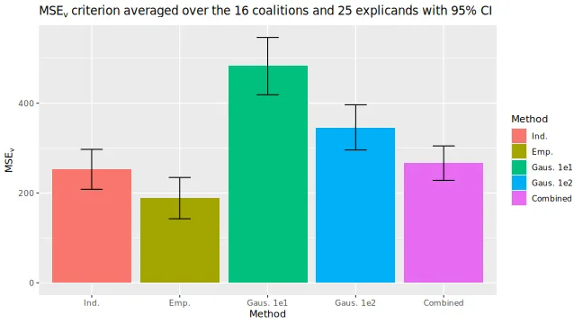

# The MSEv averaged over only the explicands for each combinations
MSEv_plots$MSEv_co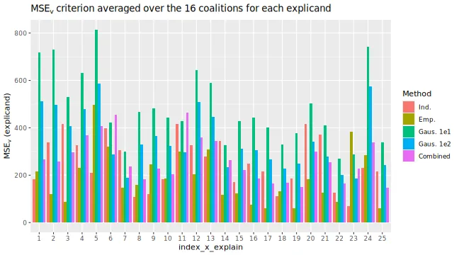mbination_bar
#> NULL

# The MSEv averaged over only the combinations for each observation/explicand
MSEv_plots$MSEv_explicand_bar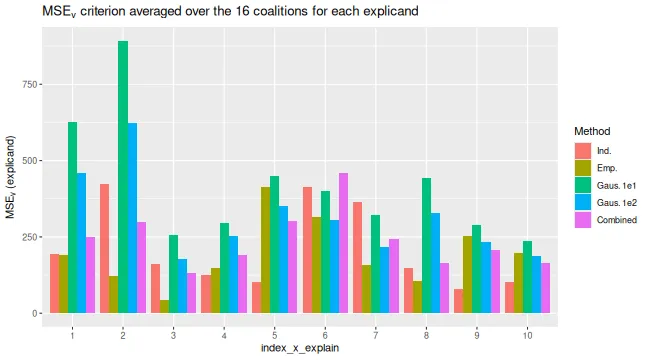

# To see which coalition S each of the `id_combination` corresponds to,
# i.e., which features that are conditions on.
explanation_list_named[[1]]$MSEv$MSEv_combination[, c("id_combination", "features")]
#> NULL

We can specify the index_x_explain and id_combination parameters in plot_MSEv_eval_crit() to only plot certain test observations and combinations, respectively.

# We can specify which test observations or combinations to plot
plot_MSEv_eval_crit(explanation_list_named,
  plot_type = "explicand",
  index_x_explain = c(1, 3:4, 6),
  CI_level = 0.95
)$MSEv_explicand_bar

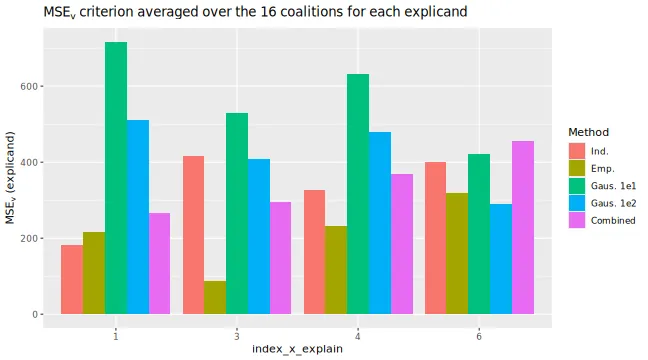
plot_MSEv_eval_crit(explanation_list_named,
  plot_type = "comb",
  id_coalition = c(3, 4, 9, 13:15),
  CI_level = 0.95
)$MSEv_combination_bar
#> NULL

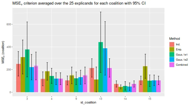
We can also alter the plots design-wise as we do in the code below.

bar_text_n_decimals <- 1
plot_MSEv_eval_crit(explanation_list_named) +
  ggplot2::scale_x_discrete(limits = rev(levels(MSEv_plots$MSEv_bar$data$Method))) +
  ggplot2::coord_flip() +
  ggplot2::scale_fill_brewer(palette = "Paired") +
  ggplot2::theme_minimal() + # This must be set before other theme calls
  ggplot2::theme(
    plot.title = ggplot2::element_text(size = 10),
    legend.position = "bottom"
  ) +
  ggplot2::geom_text(
    ggplot2::aes(label = sprintf(
      paste("%.", sprintf("%d", bar_text_n_decimals), "f", sep = ""),
      round(MSEv, bar_text_n_decimals)
    )),
    vjust = -0.35, # This number might need altering for different plots sizes
    hjust = 1.1, # This number might need altering for different plots sizes
    color = "black",
    position = ggplot2::position_dodge(0.9),
    size = 4
  )

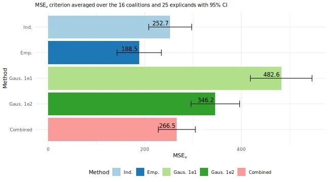
Iterative estimation

Iterative estimation is the default when computing Shapley values with six or more features (or feature groups), and can always be manually overridden by setting iterative = FALSE in the explain() function. The idea behind iterative estimation is to estimate sufficiently accurate Shapley value estimates faster. First, an initial number of coalitions is sampled, then, bootsrapping is used to estimate the variance of the Shapley values. A convergence criterion is used to determine if the variances of the Shapley values are sufficently small. If the variances are too high, we estimate the number of required samples to reach convergence, and thereby add more coalitions. The process is repeated until the variances are below the threshold. Specifics related to the iterative process and convergence criterion are set through iterative_args argument.

The convergence criterion we use is adopted from Covert and Lee (2021), and slightly modified to work for multiple observations

$$ \median_i\left(\frac{max_j \hat{\text{sd}}(\hat{\phi}_{ij}){\max_j \hat{\phi}_{ij} - \min_j \hat{\phi}_{ij}}\right), < t $$

where $\hat{\phi}_{ij}$ is the Shapley value of feature $j$ for observation $i$, and $\text{sd}(\phi_{ij})$ is the its (bootstrap) estimated standard deviation. The default value of $t$ is 0.02. Below we provide some examples of how to use the iterative estimation procedure.

library(xgboost)
library(data.table)

data("airquality")
data <- data.table::as.data.table(airquality)
data <- data[complete.cases(data), ]

x_var <- c("Solar.R", "Wind", "Temp", "Month", "Day")
y_var <- "Ozone"

ind_x_explain <- 1:6
x_train <- data[-ind_x_explain, ..x_var]
y_train <- data[-ind_x_explain, get(y_var)]
x_explain <- data[ind_x_explain, ..x_var]

# Set seed for reproducibility
set.seed(123)

# Fitting a basic xgboost model to the training data
model <- xgboost::xgboost(
  data = as.matrix(x_train),
  label = y_train,
  nround = 20,
  verbose = FALSE
)

# Specifying the phi_0, i.e. the expected prediction without any features
p0 <- mean(y_train)

# Initial explanation computation
ex <- explain(
  model = model,
  x_explain = x_explain,
  x_train = x_train,
  approach = "gaussian",
  phi0 = p0,
  iterative = TRUE,
  iterative_args = list(convergence_tol = 0.1)
)
#> Note: Feature classes extracted from the model contains NA.
#> Assuming feature classes from the data are correct.
#> Success with message:
#> max_n_coalitions is NULL or larger than or 2^n_features = 32, 
#> and is therefore set to 2^n_features = 32.
#> 
#> ── Starting `shapr::explain()` at 2024-11-21 20:44:48 ────────────────────────────────────
#> • Model class: <xgb.Booster>
#> • Approach: gaussian
#> • Iterative estimation: TRUE
#> • Number of feature-wise Shapley values: 5
#> • Number of observations to explain: 6
#> • Computations (temporary) saved at: '/tmp/RtmpCcS4cy/shapr_obj_1b8c933097162d.rds'
#> 
#> ── iterative computation started ──
#> 
#> ── Iteration 1 ───────────────────────────────────────────────────────────────────────────
#> ℹ Using 5 of 32 coalitions, 5 new.
#> 
#> ── Iteration 2 ───────────────────────────────────────────────────────────────────────────
#> ℹ Using 10 of 32 coalitions, 4 new.
#> 
#> ── Iteration 3 ───────────────────────────────────────────────────────────────────────────
#> ℹ Using 12 of 32 coalitions, 2 new.

Parallelization

The shapr package supports parallelization of the Shapley value estimation process through the future package. The parallelization is conducted over batches of v(S)-values. We therefore start by describing this batch computing.

Batch computation

The computational complexity of Shapley value based explanations grows fast in the number of features, as the number of conditional expectations one needs to estimate in the Shapley formula grows exponentially. As outlined above, the estimating of each of these conditional expectations is also computationally expensive, typically requiring estimation of a conditional probability distribution, followed by Monte Carlo integration. These computations are not only heavy for the CPU, they also require a lot of memory (RAM), which typically is a limited resource. By doing the most resource hungry computations (the computation of v(S)) in sequential batches with different feature subsets $S$, the memory usage can be significantly reduces. The user can control the number of batches by setting the two arguments extra_computation_args$max_batch_size (defaults to 10) and extra_computation_args$min_n_batches (defaults to 10).

Parallelized computation

In addition to reducing the memory consumption, the batch computing allows the computations within each batch to be performed in parallel. The parallelization in shapr::explain() is handled by the future_apply package which builds on the future environment. These packages work on all OS, allows the user to decide the parallelization backend (mutliple R procesess or forking), works directly with hpc clusters, and also supports progress updates for the parallelized task via the associated progressr package (see Verbosity and progress updates).

Note that, since it takes some time to duplicate data into different processes/machines when running in parallel, it is not always preferrable to run shapr::explain() in parallel, at least not with many parallel sessions/workers. Parallelization also increases the memory consumption proportionally, so you may want to limit the number of workers for that reason too. Below is a basic example of a parallelization with two workers.

library(future)
future::plan(multisession, workers = 2)

explanation_par <- explain(
  model = model,
  x_explain = x_explain,
  x_train = x_train,
  approach = "empirical",
  phi0 = p0
)
#> Note: Feature classes extracted from the model contains NA.
#> Assuming feature classes from the data are correct.
#> Success with message:
#> max_n_coalitions is NULL or larger than or 2^n_features = 32, 
#> and is therefore set to 2^n_features = 32.
#> 
#> ── Starting `shapr::explain()` at 2024-11-21 20:44:51 ────────────────────────────────────
#> • Model class: <xgb.Booster>
#> • Approach: empirical
#> • Iterative estimation: FALSE
#> • Number of feature-wise Shapley values: 5
#> • Number of observations to explain: 6
#> • Computations (temporary) saved at: '/tmp/RtmpCcS4cy/shapr_obj_1b8c9348628d8d.rds'
#> 
#> ── Main computation started ──
#> 
#> ℹ Using 32 of 32 coalitions.

future::plan(sequential) # To return to non-parallel computation

Verbosity and progress updates

The verbose argument controls the verbosity of the output while running explain(), and allows one or more of the strings "basic", "progress", "convergence", "shapley" and "vS_details". "basic" (default) displays basic information about the computation which is being performed, "progress displays information about where in the calculation process the function currently is, "convergence" displays information on how close to convergence the Shapley value estimates are (for iterative estimation), "shapley" displays (intermediate) Shapley value estimates and standard deviations + the final estimates, while "vS_details" displays information about the v(S) estimates for some of the approaches. If the user wants no printout, the argument can be set to NULL.

In additon, progress updates for the computation of the v(S) values are (optionally) provided through the R-package progressr. This gives the user full control over the visual appearance of these progress updates. The main reason for providing this separate progress update feature is that it integreats seamlessly with the parallelization framework future used by shapr (see Parallelization), and apparently is the only framework allowing progress updates also for parallelized tasks. These progress updates can be used in combination with, or independently of, the verbose argument.

These progress updates via progressr can be enabled for the current R-session by running the command progressr::handlers(local=TRUE), before calling explain(). To use progress updates for only a single call to explain(), one can wrap the call using progressr::with_progress as follows: progressr::with_progress({ shapr::explain() }) The default appearance of the progress updates is a basic ASCII-based horizontal progress bar. Other variants can be chosen by passing different strings to progressr::handlers(), some of which require additional packages. If you are using Rstudio, the progress can be displayed directly in the gui with progressr::handlers('rstudio') (requires the rstudioapi package). If you are running Windows, you may use the pop-up gui progress bar progressr::handlers('handler_winprogressbar'). A wrapper for progressbar of the flexible cli package, is also available progressr::handlers('cli').

For a full list of all progression handlers and the customization options available with progressr, see the progressr vignette. A full code example of using progressr with shapr is shown below:

library(progressr)
progressr::handlers(global = TRUE)
handlers("cli")
# If no progression handler is specified, the txtprogressbar is used
# Other progression handlers:
# progressr::handlers('progress') # requires the 'progress' package
# progressr::handlers('rstudio') # requires the 'rstudioapi' package
# progressr::handlers('handler_winprogressbar') # Window only
ex_progress <- explain(
  model = model,
  x_explain = x_explain,
  x_train = x_train,
  approach = "empirical",
  phi0 = p0
)

# ■■■■■■■■■■■                       32% | Estimating v(S) ETA:  2s

Advanced usage

Combined approach

In addition to letting the user select one of the five aforementioned approaches for estimating the conditional distribution of the data (i.e. approach equals either "gaussian", "copula", "empirical", "ctree", "vaeac", "categorical") or "timeseries", the package allows the user to combine the given approaches. The 'regression_surrogate' and 'regression_separate approaches are not supported for the combined approach. To simplify the usage, the flexibility is restricted such that the same approach is used when conditioning on the same number of features. This is also in line Aas, Jullum, and Løland (2021, sec. 3.4).

This can be done by setting approach equal to a character vector, where the length of the vector is one less than the number of features in the model. Consider a situation where you have trained a model that consists of 10 features, and you would like to use the "empirical" approach when you condition on 1-3 features, the "copula" approach when you condition on 4-5 features, and the "gaussian" approach when conditioning on 6 or more features. This can be applied by simply passing approach = c(rep("empirical", 3), rep("copula", 2), rep("gaussian", 4)), i.e. approach[i] determines which method to use when conditioning on i features. Conditioning on all features needs no approach as that is given by the complete prediction itself, and should thus not be part of the vector.

The code below exemplifies this approach for a case where there are four features, using "empirical", "copula" and "gaussian" when conditioning on respectively 1, 2 and 3 features.

library(xgboost)
library(data.table)

data("airquality")
data <- data.table::as.data.table(airquality)
data <- data[complete.cases(data), ]

x_var <- c("Solar.R", "Wind", "Temp", "Month")
y_var <- "Ozone"

ind_x_explain <- 1:6
x_train <- data[-ind_x_explain, ..x_var]
y_train <- data[-ind_x_explain, get(y_var)]
x_explain <- data[ind_x_explain, ..x_var]

# Set seed for reproducibility
set.seed(123)

# Fitting a basic xgboost model to the training data
model <- xgboost::xgboost(
  data = as.matrix(x_train),
  label = y_train,
  nround = 20,
  verbose = FALSE
)

# Specifying the phi_0, i.e. the expected prediction without any features
p0 <- mean(y_train)


# Use the combined approach
explanation_combined <- explain(
  model = model,
  x_explain = x_explain,
  x_train = x_train,
  approach = c("empirical", "copula", "gaussian"),
  phi0 = p0
)
#> Note: Feature classes extracted from the model contains NA.
#> Assuming feature classes from the data are correct.
#> Success with message:
#> max_n_coalitions is NULL or larger than or 2^n_features = 16, 
#> and is therefore set to 2^n_features = 16.
#> 
#> ── Starting `shapr::explain()` at 2024-11-21 20:44:54 ────────────────────────────────────
#> • Model class: <xgb.Booster>
#> • Approach: empirical, copula, and gaussian
#> • Iterative estimation: FALSE
#> • Number of feature-wise Shapley values: 4
#> • Number of observations to explain: 6
#> • Computations (temporary) saved at: '/tmp/RtmpCcS4cy/shapr_obj_1b8c936a965bd5.rds'
#> 
#> ── Main computation started ──
#> 
#> ℹ Using 16 of 16 coalitions.
# Plot the resulting explanations for observations 1 and 6, excluding
# the no-covariate effect
plot(explanation_combined, bar_plot_phi0 = FALSE, index_x_explain = c(1, 6))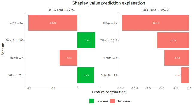

As a second example using "ctree" to condition on 1 and 2 features, and "empirical" when conditioning on 3 features:

# Use the combined approach
explanation_combined <- explain(
  model = model,
  x_explain = x_explain,
  x_train = x_train,
  approach = c("ctree", "ctree", "empirical"),
  phi0 = p0
)
#> Note: Feature classes extracted from the model contains NA.
#> Assuming feature classes from the data are correct.
#> Success with message:
#> max_n_coalitions is NULL or larger than or 2^n_features = 16, 
#> and is therefore set to 2^n_features = 16.
#> 
#> ── Starting `shapr::explain()` at 2024-11-21 20:44:57 ────────────────────────────────────
#> • Model class: <xgb.Booster>
#> • Approach: ctree, ctree, and empirical
#> • Iterative estimation: FALSE
#> • Number of feature-wise Shapley values: 4
#> • Number of observations to explain: 6
#> • Computations (temporary) saved at: '/tmp/RtmpCcS4cy/shapr_obj_1b8c93207aeb18.rds'
#> 
#> ── Main computation started ──
#> 
#> ℹ Using 16 of 16 coalitions.

Explain groups of features

In some cases, especially when the number of features is very large, it may be more appropriate to explain predictions in terms of groups of features instead of single features, see (Jullum, Redelmeier, and Aas (2021)) for intuition and real world examples. Explaining prediction in terms of groups of features is very easy using shapr:

# Define the feature groups
group_list <- list(
  A = c("Temp", "Month"),
  B = c("Wind", "Solar.R")
)

# Use the empirical approach
explanation_group <- explain(
  model = model,
  x_explain = x_explain,
  x_train = x_train,
  approach = "empirical",
  phi0 = p0,
  group = group_list
)
#> Note: Feature classes extracted from the model contains NA.
#> Assuming feature classes from the data are correct.
#> Success with message:
#> max_n_coalitions is NULL or larger than or 2^n_groups = 4, 
#> and is therefore set to 2^n_groups = 4.
#> 
#> ── Starting `shapr::explain()` at 2024-11-21 20:44:59 ────────────────────────────────────
#> • Model class: <xgb.Booster>
#> • Approach: empirical
#> • Iterative estimation: FALSE
#> • Number of group-wise Shapley values: 2
#> • Number of observations to explain: 6
#> • Computations (temporary) saved at: '/tmp/RtmpCcS4cy/shapr_obj_1b8c93241851b9.rds'
#> 
#> ── Main computation started ──
#> 
#> ℹ Using 4 of 4 coalitions.
# Prints the group-wise explanations
explanation_group
#>    explain_id  none      A        B
#>         <int> <num>  <num>    <num>
#> 1:          1 43.09 -29.25  16.0731
#> 2:          2 43.09 -15.17  -7.8373
#> 3:          3 43.09 -13.07 -10.8778
#> 4:          4 43.09 -17.47   0.6653
#> 5:          5 43.09 -28.27   3.5289
#> 6:          6 43.09 -20.59  -3.3793
# Plots the group-wise explanations
plot(explanation_group, bar_plot_phi0 = TRUE, index_x_explain = c(1, 6))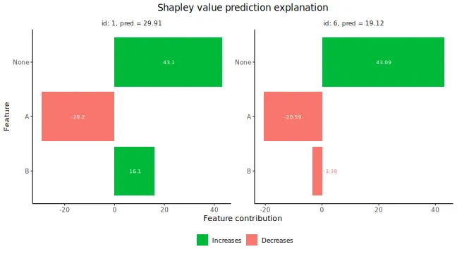

Explain custom models

shapr currently natively supports explanation of predictions from models fitted with the following functions:

• stats::lm
• stats::glm
• ranger::ranger
• mgcv::gam
• xgboost::xgboost/xgboost::xgb.train
• workflows::workflow

Any continuous response regression model or binary classification model of these model classes, can be explained with the package directly as exemplified above, while we give an example for the workflows::workflow in the tidymodels/workflows section. Moreover, essentially any feature dependent prediction model can be explained by the package by specifying two (or one) simple additional functions for your model.

The first function is predict_model, taking the model and data (as a matrix or data.frame/data.table) as input and outputting the corresponding prediction as a numeric vector. The second (optional, but highly recommended) function is get_model_specs, taking the model as input and outputting a list with the following elements: labels (vector with the feature names to compute Shapley values for), classes (a named vector with the labels as names and the class type as elements), factor_levels (a named list with the labels as names and vectors with the factor levels as elements (NULL if the feature is not a factor)). The get_model_specs function is used to check that the format of the data passed to explain have the correct format in terms of the necessary feature columns being available and having the correct class/attributes. It is highly recommended to do such checks in order to ensure correct usage of explain. If, for some reason, such checking is not desirable, one does not have to provide the get_model_specs function. This will, however, throw a warning that all feature consistency checking against the model is disabled.

Once the above functions are created, you can explain predictions from this model as before by passing the functions through the input arguments predict_model and get_model_specs of explain().

These functions can be made general enough to handle all supported model types of that class, or they can be made minimal, possibly only allowing explanation of the specific version of the model class at hand. Below we give examples of both full support versions of these functions and a minimal version which skips the get_model_specs function. We do this for the gbm model class from the gbm package, fitted to the same airquality data set as used above.

library(gbm)

formula_gbm <- as.formula(paste0(y_var, "~", paste0(x_var, collapse = "+")))
# Fitting a gbm model
set.seed(825)
model_gbm <- gbm::gbm(
  formula_gbm,
  data = cbind(x_train, Ozone = y_train),
  distribution = "gaussian"
)

#### Full feature versions of the three required model functions ####
MY_predict_model <- function(x, newdata) {
  if (!requireNamespace("gbm", quietly = TRUE)) {
    stop("The gbm package is required for predicting train models")
  }
  model_type <- ifelse(
    x$distribution$name %in% c("bernoulli", "adaboost"),
    "classification",
    "regression"
  )
  if (model_type == "classification") {
    predict(x, as.data.frame(newdata), type = "response", n.trees = x$n.trees)
  } else {
    predict(x, as.data.frame(newdata), n.trees = x$n.trees)
  }
}
MY_get_model_specs <- function(x) {
  feature_specs <- list()
  feature_specs$labels <- labels(x$Terms)
  m <- length(feature_specs$labels)
  feature_specs$classes <- attr(x$Terms, "dataClasses")[-1]
  feature_specs$factor_levels <- setNames(vector("list", m), feature_specs$labels)
  feature_specs$factor_levels[feature_specs$classes == "factor"] <- NA # model object doesn't contain factor levels info
  return(feature_specs)
}

# Compute the Shapley values
set.seed(123)
p0 <- mean(y_train)
explanation_custom <- explain(
  model = model_gbm,
  x_explain = x_explain,
  x_train = x_train,
  approach = "empirical",
  phi0 = p0,
  predict_model = MY_predict_model,
  get_model_specs = MY_get_model_specs
)
#> Success with message:
#> max_n_coalitions is NULL or larger than or 2^n_features = 16, 
#> and is therefore set to 2^n_features = 16.
#> 
#> ── Starting `shapr::explain()` at 2024-11-21 20:45:01 ────────────────────────────────────
#> • Model class: <gbm>
#> • Approach: empirical
#> • Iterative estimation: FALSE
#> • Number of feature-wise Shapley values: 4
#> • Number of observations to explain: 6
#> • Computations (temporary) saved at: '/tmp/RtmpCcS4cy/shapr_obj_1b8c933748f819.rds'
#> 
#> ── Main computation started ──
#> 
#> ℹ Using 16 of 16 coalitions.

# Plot results
plot(explanation_custom, index_x_explain = c(1, 6))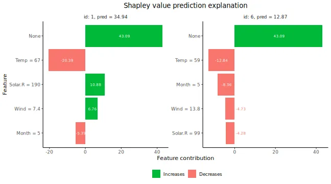

#### Minimal version of the custom model setup ####
# Note: Working only for this exact version of the model class
# Avoiding to define get_model_specs skips all feature
# consistency checking between your data and model
MY_MINIMAL_predict_model <- function(x, newdata) {
  predict(x, as.data.frame(newdata), n.trees = x$n.trees)
}

# Compute the Shapley values
set.seed(123)
explanation_custom_minimal <- explain(
  model = model_gbm,
  x_explain = x_explain,
  x_train = x_train,
  approach = "empirical",
  phi0 = p0,
  predict_model = MY_MINIMAL_predict_model
)
#> Note: You passed a model to explain() which is not natively supported, and did not supply a 'get_model_specs' function to explain().
#> Consistency checks between model and data is therefore disabled.
#> Success with message:
#> max_n_coalitions is NULL or larger than or 2^n_features = 16, 
#> and is therefore set to 2^n_features = 16.
#> 
#> ── Starting `shapr::explain()` at 2024-11-21 20:45:07 ────────────────────────────────────
#> • Model class: <gbm>
#> • Approach: empirical
#> • Iterative estimation: FALSE
#> • Number of feature-wise Shapley values: 4
#> • Number of observations to explain: 6
#> • Computations (temporary) saved at: '/tmp/RtmpCcS4cy/shapr_obj_1b8c9344b0ff8e.rds'
#> 
#> ── Main computation started ──
#> 
#> ℹ Using 16 of 16 coalitions.

# Plot results
plot(explanation_custom_minimal, index_x_explain = c(1, 6))

Tidymodels and workflows

In this section, we demonstrate how to use shapr to explain tidymodels models fitted using workflows. In the example above, we directly used the xgboost package to fit the xgboost model. However, we can also fit the xgboost model using the tidymodels package. These fits will be identical as tidymodels calls xgboost internally. which we demonstrate in the example below. Note that we can replace xgboost (i.e., parsnip::boost_tree) with any other fitted tidymodels in the workflows procedure outlined below.

# Fitting a basic xgboost model to the training data using tidymodels
set.seed(123) # Set the same seed as above
all_var <- c(y_var, x_var)
train <- data[-ind_x_explain, ..all_var]

# Fitting the `tidymodels` model using `workflows`
model_tidymodels <- parsnip::fit(
  workflows::add_recipe(
    workflows::add_model(
      workflows::workflow(),
      parsnip::boost_tree(trees = 20, engine = "xgboost", mode = "regression")
    ),
    recipes::recipe(Ozone ~ ., data = train)
  ),
  data = train
)

# # We can also specify the same model using pipes `%>%` by (if pipes are installed/loaded)
# model_tidymodels <-
#   workflows::workflow() %>%
#   workflows::add_model(parsnip::boost_tree(trees = 20, engine = "xgboost", mode = "regression")) %>%
#   workflows::add_recipe(recipes::recipe(Ozone ~ ., data = train)) %>%
#   parsnip::fit(data = train)

# See that the output of the two models are identical
all.equal(predict(model_tidymodels, x_train)$.pred, predict(model, as.matrix(x_train)))
#> [1] TRUE

# Create the Shapley values for the tidymodels version
explanation_tidymodels <- explain(
  model = model_tidymodels,
  x_explain = x_explain,
  x_train = x_train,
  approach = "empirical",
  phi0 = p0
)
#> Success with message:
#> max_n_coalitions is NULL or larger than or 2^n_features = 16, 
#> and is therefore set to 2^n_features = 16.
#> 
#> ── Starting `shapr::explain()` at 2024-11-21 20:45:13 ────────────────────────────────────
#> • Model class: <workflow>
#> • Approach: empirical
#> • Iterative estimation: FALSE
#> • Number of feature-wise Shapley values: 4
#> • Number of observations to explain: 6
#> • Computations (temporary) saved at: '/tmp/RtmpCcS4cy/shapr_obj_1b8c93476395f2.rds'
#> 
#> ── Main computation started ──
#> 
#> ℹ Using 16 of 16 coalitions.

# See that the Shapley value explanations are identical too
all.equal(explanation$shapley_values_est, explanation_tidymodels$shapley_values_est)
#> [1] TRUE

The parameters of the vaeac approach

The vaeac approach is a very flexible method that supports mixed data. The main parameters are the the number of layers in the networks (vaeac.depth), the width of the layers (vaeac.width), the number of dimensions in the latent space (vaeac.latent_dim), the activation function between the layers in the networks (vaeac.activation_function), the learning rate in the ADAM optimizer (vaeac.lr), the number of vaeac models to initiate to remedy poorly initiated model parameter values (vaeac.n_vaeacs_initialize), and the number of learning epochs (vaeac.epochs). Call ?shapr::setup_approach.vaeac for a more detailed description of the parameters.

There are additional extra parameters which can be set by including a named list in the call to the explain() function. For example, we can the change the batch size to 32 by including vaeac.extra_parameters = list(vaeac.batch_size = 32) as a parameter in the call the explain() function. See ?shapr::vaeac_get_extra_para_default for a description of the possible extra parameters to the vaeac approach. The main parameters are directly entered to the explain() function, while the extra parameters are included in a named list called vaeac.extra_parameters.

explanation_vaeac <- explain(
  model = model,
  x_explain = x_explain,
  x_train = x_train,
  approach = "vaeac",
  phi0 = p0,
  n_MC_samples = 100,
  vaeac.width = 16,
  vaeac.depth = 2,
  vaeac.epochs = 3,
  vaeac.n_vaeacs_initialize = 2
)
#> Note: Feature classes extracted from the model contains NA.
#> Assuming feature classes from the data are correct.
#> Success with message:
#> max_n_coalitions is NULL or larger than or 2^n_features = 16, 
#> and is therefore set to 2^n_features = 16.
#> 
#> ── Starting `shapr::explain()` at 2024-11-21 20:45:19 ────────────────────────────────────
#> • Model class: <xgb.Booster>
#> • Approach: vaeac
#> • Iterative estimation: FALSE
#> • Number of feature-wise Shapley values: 4
#> • Number of observations to explain: 6
#> • Computations (temporary) saved at: '/tmp/RtmpCcS4cy/shapr_obj_1b8c932349a0b1.rds'
#> 
#> ── Main computation started ──
#> 
#> ℹ Using 16 of 16 coalitions.

Can look at the training and validation error for the trained vaeac model and see that vaeac.epochs = 3 is likely to few epochs as it still seems like the vaeac model is learning.

# Look at the training and validation errors.
plot_vaeac_eval_crit(list("Vaeac 3 epochs" = explanation_vaeac), plot_type = "method")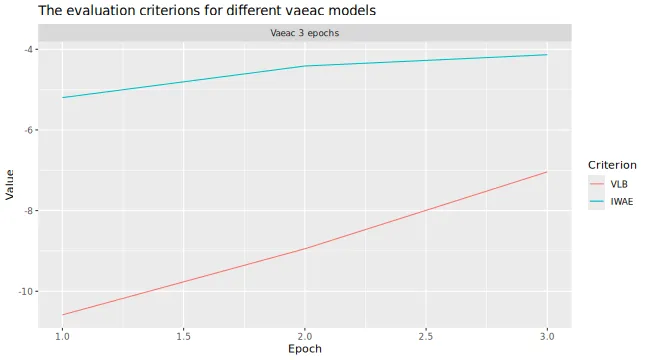

Early stopping

If we are uncertain about the choice of vaeac.epochs, we can rather use vaeac with early stopping. We will then set vaeac.epochs to a large number which will act as a maximum number of allowed epochs and in the vaeac.extra_parameters list, we set vaeac.epochs_early_stopping the number of epochs we allow the vaeac model to not improve its validation score. That is, if vaeac.epochs_early_stopping = 2, then vaeac will stop the training procedure if there has been no improvement in the validation score for 2 consecutive epochs, of if vaeac.epochs is reached. Note that if using early stopping and progress updates simultaneously, then the estimated timer remaining will obviously be incorrect if early stopping is applied. Furthermore, a value of 2 is too low for real world applications, but we set it so low here to make the vignette faster to build.

explanation_vaeac_early_stop <- explain(
  model = model,
  x_explain = x_explain,
  x_train = x_train,
  approach = "vaeac",
  phi0 = p0,
  n_MC_samples = 100,
  vaeac.width = 16,
  vaeac.depth = 2,
  vaeac.epochs = 1000, # Set it to a large number
  vaeac.n_vaeacs_initialize = 2,
  vaeac.extra_parameters = list(vaeac.epochs_early_stopping = 2)
)
#> Note: Feature classes extracted from the model contains NA.
#> Assuming feature classes from the data are correct.
#> Success with message:
#> max_n_coalitions is NULL or larger than or 2^n_features = 16, 
#> and is therefore set to 2^n_features = 16.
#> 
#> ── Starting `shapr::explain()` at 2024-11-21 20:45:34 ────────────────────────────────────
#> • Model class: <xgb.Booster>
#> • Approach: vaeac
#> • Iterative estimation: FALSE
#> • Number of feature-wise Shapley values: 4
#> • Number of observations to explain: 6
#> • Computations (temporary) saved at: '/tmp/RtmpCcS4cy/shapr_obj_1b8c9361ebec61.rds'
#> 
#> ── Main computation started ──
#> 
#> ℹ Using 16 of 16 coalitions.

Can compare with the previous version and see that the results are more stable now.

# Look at the training and validation errors.
plot_vaeac_eval_crit(
  list("Vaeac 3 epochs" = explanation_vaeac, "Vaeac early stopping" = explanation_vaeac_early_stop),
  plot_type = "method"
)

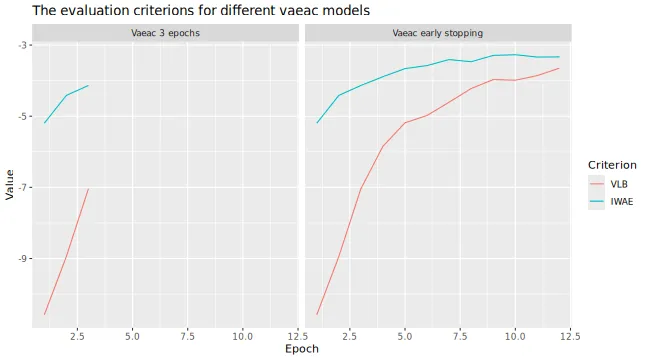
Can also compare the $MSE_{v}$ evaluation scores.

plot_MSEv_eval_crit(list("Vaeac 3 epochs" = explanation_vaeac, "Vaeac early stopping" = explanation_vaeac_early_stop))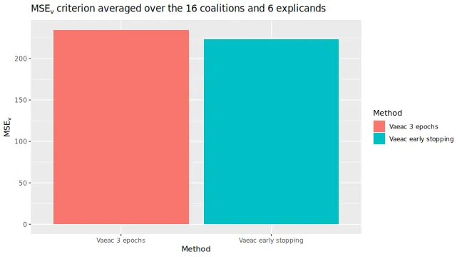

Continued computation

In this section, we demonstrate how to continue to improve estimation accuracy with additional coalition samples, from a previous Shapley value computation based on shapr::explain() with the iterative estimation procedure. This can be done either by passing an existing object of class shapr, or by passing a string with the path to the intermediately saved results. The latter is found at SHAPR_OBJ$saving_path, defaults to a temporary folder, and is updated after each iteration. This can be particularly handy for long-running computations.

# First we run the computation with the iterative estimation procedure for a limited number of coalition samples
library(xgboost)
library(data.table)

data("airquality")
data <- data.table::as.data.table(airquality)
data <- data[complete.cases(data), ]

x_var <- c("Solar.R", "Wind", "Temp", "Month", "Day")
y_var <- "Ozone"

ind_x_explain <- 1:6
x_train <- data[-ind_x_explain, ..x_var]
y_train <- data[-ind_x_explain, get(y_var)]
x_explain <- data[ind_x_explain, ..x_var]

# Set seed for reproducibility
set.seed(123)

# Fitting a basic xgboost model to the training data
model <- xgboost::xgboost(
  data = as.matrix(x_train),
  label = y_train,
  nround = 20,
  verbose = FALSE
)

# Specifying the phi_0, i.e. the expected prediction without any features
p0 <- mean(y_train)

# Initial explanation computation
ex_init <- explain(
  model = model,
  x_explain = x_explain,
  x_train = x_train,
  approach = "gaussian",
  phi0 = p0,
  max_n_coalitions = 20,
  iterative = TRUE
)
#> Note: Feature classes extracted from the model contains NA.
#> Assuming feature classes from the data are correct.
#> 
#> ── Starting `shapr::explain()` at 2024-11-21 20:45:57 ────────────────────────────────────
#> • Model class: <xgb.Booster>
#> • Approach: gaussian
#> • Iterative estimation: TRUE
#> • Number of feature-wise Shapley values: 5
#> • Number of observations to explain: 6
#> • Computations (temporary) saved at: '/tmp/RtmpCcS4cy/shapr_obj_1b8c93667c79.rds'
#> 
#> ── iterative computation started ──
#> 
#> ── Iteration 1 ───────────────────────────────────────────────────────────────────────────
#> ℹ Using 5 of 32 coalitions, 5 new.
#> 
#> ── Iteration 2 ───────────────────────────────────────────────────────────────────────────
#> ℹ Using 10 of 32 coalitions, 4 new.
#> 
#> ── Iteration 3 ───────────────────────────────────────────────────────────────────────────
#> ℹ Using 12 of 32 coalitions, 2 new.
#> 
#> ── Iteration 4 ───────────────────────────────────────────────────────────────────────────
#> ℹ Using 16 of 32 coalitions, 4 new.
#> 
#> ── Iteration 5 ───────────────────────────────────────────────────────────────────────────
#> ℹ Using 18 of 32 coalitions, 2 new.

# Using the ex_init object to continue the computation with 5 more coalition samples
ex_further <- explain(
  model = model,
  x_explain = x_explain,
  x_train = x_train,
  approach = "gaussian",
  phi0 = p0,
  max_n_coalitions = 25,
  iterative_args = list(convergence_tol = 0.005), # Decrease the convergence threshold
  prev_shapr_object = ex_init
)
#> Note: Feature classes extracted from the model contains NA.
#> Assuming feature classes from the data are correct.
#> 
#> ── Starting `shapr::explain()` at 2024-11-21 20:46:01 ────────────────────────────────────
#> • Model class: <xgb.Booster>
#> • Approach: gaussian
#> • Iterative estimation: FALSE
#> • Number of feature-wise Shapley values: 5
#> • Number of observations to explain: 6
#> • Computations (temporary) saved at: '/tmp/RtmpCcS4cy/shapr_obj_1b8c937cd2ac71.rds'
#> 
#> ── Main computation started ──
#> 
#> ℹ Using 24 of 32 coalitions.

print(ex_further$saving_path)
#> [1] "/tmp/RtmpCcS4cy/shapr_obj_1b8c937cd2ac71.rds"

# Using the ex_init object to continue the computation for the remaining coalition samples
# but this time using the path to the saved intermediate estimation object
ex_even_further <- explain(
  model = model,
  x_explain = x_explain,
  x_train = x_train,
  approach = "gaussian",
  phi0 = p0,
  max_n_coalitions = NULL,
  prev_shapr_object = ex_further$saving_path
)
#> Note: Feature classes extracted from the model contains NA.
#> Assuming feature classes from the data are correct.
#> Success with message:
#> max_n_coalitions is NULL or larger than or 2^n_features = 32, 
#> and is therefore set to 2^n_features = 32.
#> 
#> ── Starting `shapr::explain()` at 2024-11-21 20:46:02 ────────────────────────────────────
#> • Model class: <xgb.Booster>
#> • Approach: gaussian
#> • Iterative estimation: FALSE
#> • Number of feature-wise Shapley values: 5
#> • Number of observations to explain: 6
#> • Computations (temporary) saved at: '/tmp/RtmpCcS4cy/shapr_obj_1b8c936aa37ec8.rds'
#> 
#> ── Main computation started ──
#> 
#> ℹ Using 32 of 32 coalitions.

Explaining a forecasting model using explain_forecast

shapr provides a specific function, explain_forecast, to explain forecasts from time series models, at one or more steps into the future. The main difference compared to explain is that the data is supplied as (set of) time series, in addition to index arguments (train_idx and explain_idx) specifying which time points that represents the train and explain parts of the data. See ?explain_forecast for more information.

To demonstrate how to use the function, 500 observations are generated which follow an AR(1) structure, i.e. $y_t = 0.5 y_{t-1} + \varepsilon_t$. To this data an arima model of order (2, 0, 0) is fitted, and we therefore would like to explain the forecasts in terms of the two previous lags of the time series. This is is specified through the argument explain_y_lags = 2. Note that some models may also put restrictions on the amount of data required to make a forecast. The AR(2) model we used there, for instance, requires two previous time point to make a forecast.

In the example, two separate forecasts, each three steps ahead, are explained. To set the starting points of the two forecasts, explain_idx is set to 499:500. This means that one forecast of $t = (500, 501, 502)$ and another of $t = (501, 502, 503)$, will be explained. In other words, explain_idx tells shapr at which points in time data was available up until, when making the forecast to explain.

In the same way, train_idx denotes the points in time used to estimate the conditional expectations used to explain the different forecasts. Note that since we want to explain the forecasts in terms of the two previous lags (explain_y_lags = 2), the smallest value of train_idx must also be 2, because at time $t = 1$ there was only a single observation available.

Since the data is stationary, the mean of the data is used as value of phi0 (i.e. $\phi_0$). This can however be chosen differently depending on the data and application.

For a multivariate model such as a VAR (Vector AutoRegressive model), it may be more interesting to explain the impact of each variable, rather than each lag of each variable. This can be done by setting group_lags = TRUE.

# Simulate time series data with AR(1)-structure.
set.seed(1)
data_ts <- data.frame(Y = arima.sim(list(order = c(1, 0, 0), ar = .5), n = 500))
data_ts <- data.table::as.data.table(data_ts)

# Fit an ARIMA(2, 0, 0) model.
arima_model <- arima(data_ts, order = c(2, 0, 0))

# Set prediction zero as the mean of the data for each forecast point.
p0_ar <- rep(mean(data_ts$Y), 3)

# Explain forecasts from points t = 499 and t = 500.
explain_idx <- 499:500

explanation_forecast <- explain_forecast(
  model = arima_model,
  y = data_ts,
  train_idx = 2:498,
  explain_idx = 499:500,
  explain_y_lags = 2,
  horizon = 3,
  approach = "empirical",
  phi0 = p0_ar,
  group_lags = FALSE
)
#> Note: Feature names extracted from the model contains NA.
#> Consistency checks between model and data is therefore disabled.
#> Success with message:
#> max_n_coalitions is NULL or larger than or 2^n_features = 4, 
#> and is therefore set to 2^n_features = 4.
#> 
#> ── Starting `shapr::explain()` at 2024-11-21 20:46:03 ────────────────────────────────────
#> • Model class: <Arima>
#> • Approach: empirical
#> • Iterative estimation: FALSE
#> • Number of feature-wise Shapley values: 2
#> • Number of observations to explain: 2
#> • Computations (temporary) saved at: '/tmp/RtmpCcS4cy/shapr_obj_1b8c931eee7980.rds'
#> 
#> ── Main computation started ──
#> 
#> ℹ Using 4 of 4 coalitions.
explanation_forecast
#>    explain_idx horizon    none     Y.1      Y.2
#>          <int>   <int>   <num>   <num>    <num>
#> 1:         499       1 0.04018  0.5053 -0.07659
#> 2:         500       1 0.04018 -0.3622  0.02497
#> 3:         499       2 0.04018  0.5053 -0.07659
#> 4:         500       2 0.04018 -0.3622  0.02497
#> 5:         499       3 0.04018  0.5053 -0.07659
#> 6:         500       3 0.04018 -0.3622  0.02497

Note that for a multivariate model such as a VAR (Vector AutoRegressive model), or for models also including several exogenous variables, it may be of more informative to explain the impact of each variable, rather than each lag of each variable. This can be done by setting group_lags = TRUE. This does not make sense for this model, however, as that would result in decomposing the forecast into a single group.

We now give a more hands on example of how to use the explain_forecast function. Say that we have an AR(2) model which describes the change over time of the variable Temp in the dataset airquality. It seems reasonable to assume that the temperature today should affect the temperature tomorrow. To a lesser extent, we may also suggest that the temperature today should also have an impact on that of the day after tomorrow.

We start by building our AR(2) model, naming it model_ar_temp. This model is then used to make a forecast of the temperature of the day that comes after the last day in the data, this forecast starts from index 153.

data_ts2 <- data.table::as.data.table(airquality)

model_ar_temp <- ar(data_ts2$Temp, order = 2)

predict(model_ar_temp, n.ahead = 2)$pred
#> Time Series:
#> Start = 154 
#> End = 155 
#> Frequency = 1 
#> [1] 71.081 71.524

First, we pass the model and the data as model and y. Since we have an AR(2) model, we want to explain the forecasts in terms of the two previous lags, whihc we specify with explain_y_lags = 2. Then, we let shapr know which time indices to use as training data through the argument train_idx. We use 2:152, meaning that we skip the first index, as we want to explain the two previous lags. Letting the training indices go up until 152 means that every point in time except the first and last will be used as training data.

The last index, 153 is passed as the argument explain_idx, which means that we want to explain a forecast made from time point 153 in the data. The argument horizon is set to 2 in order to explain a forecast of length 2.

The argument phi0 is set to the mean of the time series, and is repeated two times. Each value of phi0 is the baseline for each forecast horizon. In our example, we assume that given no effect from the two lags, the temperature would just be the average during the observed period. Finally, we opt to not group the lags by setting group_lags to FALSE. This means that lag 1 and 2 will be explained separately. Grouping lags may be more interesting to do in a model with multiple variables, as it is then possible to explain each variable separately.

explanation_forecast <- explain_forecast(
  model = model_ar_temp,
  y = data_ts2[, "Temp"],
  train_idx = 2:152,
  explain_idx = 153,
  explain_y_lags = 2,
  horizon = 2,
  approach = "empirical",
  phi0 = rep(mean(data$Temp), 2),
  group_lags = FALSE
)
#> Note: Feature names extracted from the model contains NA.
#> Consistency checks between model and data is therefore disabled.
#> Success with message:
#> max_n_coalitions is NULL or larger than or 2^n_features = 4, 
#> and is therefore set to 2^n_features = 4.
#> 
#> ── Starting `shapr::explain()` at 2024-11-21 20:46:05 ────────────────────────────────────
#> • Model class: <ar>
#> • Approach: empirical
#> • Iterative estimation: FALSE
#> • Number of feature-wise Shapley values: 2
#> • Number of observations to explain: 1
#> • Computations (temporary) saved at: '/tmp/RtmpCcS4cy/shapr_obj_1b8c9360892168.rds'
#> 
#> ── Main computation started ──
#> 
#> ℹ Using 4 of 4 coalitions.

print(explanation_forecast)
#>    explain_idx horizon  none Temp.1 Temp.2
#>          <num>   <num> <num>  <num>  <num>
#> 1:         153       1 77.79 -6.578 -0.134
#> 2:         153       2 77.79 -5.980 -0.288

The results are presented per value of explain_idx and forecast horizon. We can see that the mean temperature was around 77.9 degrees. At horizon 1, the first lag in the model caused it to be 6.6 degrees lower, and the second lag had just a minor effect. At horizon 2, the first lag has a slightly smaller negative impact, and the second lag has a slightly larger impact.

It is also possible to explain a forecasting model which uses exogenous regressors. The previous example is expanded to use an ARIMA(2,0,0) model with Wind as an exogenous regressor. Since the exogenous regressor must be available for the predicted time points, the model is just fit on the 151 first observations, leaving two observations of Wind to be used as exogenous values during the prediction phase.

data_ts3 <- data.table::as.data.table(airquality)

data_fit <- data_ts3[seq_len(151), ]

model_arimax_temp <- arima(data_fit$Temp, order = c(2, 0, 0), xreg = data_fit$Wind)

newxreg <- data_ts3[-seq_len(151), "Wind", drop = FALSE]

predict(model_arimax_temp, n.ahead = 2, newxreg = newxreg)$pred
#> Time Series:
#> Start = 152 
#> End = 153 
#> Frequency = 1 
#> [1] 77.500 76.381

The shapr package can then explain not only the two autoregressive lags, but also the single lag of the exogenous regressor. In order to do so, the Wind variable is passed as the argument xreg, and explain_xreg_lags is set to 1. Notice how only the first 151 observations are used for y and all 153 are used for xreg. This makes it possible for shapr to not only explain the effect of the first lag of the exogenous variable, but also the contemporary effect during the forecasting period.

explanation_forecast <- explain_forecast(
  model = model_ar_temp,
  y = data_fit[, "Temp"],
  xreg = data_ts3[, "Wind"],
  train_idx = 2:150,
  explain_idx = 151,
  explain_y_lags = 2,
  explain_xreg_lags = 1,
  horizon = 2,
  approach = "empirical",
  phi0 = rep(mean(data_fit$Temp), 2),
  group_lags = FALSE
)
#> Note: Feature names extracted from the model contains NA.
#> Consistency checks between model and data is therefore disabled.
#> Success with message:
#> max_n_coalitions is NULL or larger than or 2^n_features = 32, 
#> and is therefore set to 2^n_features = 32.
#> 
#> ── Starting `shapr::explain()` at 2024-11-21 20:46:07 ────────────────────────────────────
#> • Model class: <ar>
#> • Approach: empirical
#> • Iterative estimation: FALSE
#> • Number of feature-wise Shapley values: 5
#> • Number of observations to explain: 1
#> • Computations (temporary) saved at: '/tmp/RtmpCcS4cy/shapr_obj_1b8c93398eb42e.rds'
#> 
#> ── Main computation started ──
#> 
#> ℹ Using 32 of 32 coalitions.

print(explanation_forecast$shapley_values_est)
#>    explain_idx horizon  none   Temp.1   Temp.2  Wind.1  Wind.F1  Wind.F2
#>          <num>   <num> <num>    <num>    <num>   <num>    <num>    <num>
#> 1:         151       1 77.96 -0.67793 -0.67340 -1.2688 0.493408       NA
#> 2:         151       2 77.96  0.39968 -0.50059 -1.4655 0.065913 -0.47422

References

Aas, Kjersti, Martin Jullum, and Anders Løland. 2021. “Explaining Individual Predictions When Features Are Dependent: More Accurate Approximations to Shapley Values.” Artificial Intelligence 298.

Covert, Ian, and Su-In Lee. 2021. “Improving Kernelshap: Practical Shapley Value Estimation Using Linear Regression.” In International Conference on Artificial Intelligence and Statistics, 3457–65. PMLR.

Covert, Ian, Scott M Lundberg, and Su-In Lee. 2020. “Understanding Global Feature Contributions with Additive Importance Measures.” Advances in Neural Information Processing Systems 33: 17212–23.

Falbel, Daniel, and Javier Luraschi. 2023. Torch: Tensors and Neural Networks with ’GPU’ Acceleration. https://CRAN.R-project.org/package=torch.

Frye, Christopher, Damien de Mijolla, Tom Begley, Laurence Cowton, Megan Stanley, and Ilya Feige. 2021. “Shapley Explainability on the Data Manifold.” In International Conference on Learning Representations.

Hothorn, Torsten, Kurt Hornik, and Achim Zeileis. 2006. “Unbiased Recursive Partitioning: A Conditional Inference Framework.” Journal of Computational and Graphical Statistics 15 (3): 651–74.

Hothorn, Torsten, and Achim Zeileis. 2015. “partykit: A Modular Toolkit for Recursive Partytioning in R.” Journal of Machine Learning Research 16: 3905–9.

Jullum, Martin, Annabelle Redelmeier, and Kjersti Aas. 2021. “Efficient and Simple Prediction Explanations with groupShapley: A Practical Perspective.” In Proceedings of the 2nd Italian Workshop on Explainable Artificial Intelligence, 28–43. CEUR Workshop Proceedings.

Kingma, Diederik P., and Max Welling. 2014. “Auto-Encoding Variational Bayes.” In 2nd International Conference on Learning Representations, ICLR 2014, Banff, AB, Canada, April 14-16, 2014, Conference Track Proceedings.

Lundberg, Scott M, and Su-In Lee. 2017. “A Unified Approach to Interpreting Model Predictions.” In Advances in Neural Information Processing Systems, 4765–74.

Olsen, Lars Henry Berge, Ingrid Kristine Glad, Martin Jullum, and Kjersti Aas. 2022. “Using Shapley Values and Variational Autoencoders to Explain Predictive Models with Dependent Mixed Features.” Journal of Machine Learning Research 23 (213): 1–51.

———. 2024. “A Comparative Study of Methods for Estimating Model-Agnostic Shapley Value Explanations.” Data Mining and Knowledge Discovery, 1–48.

Redelmeier, Annabelle, Martin Jullum, and Kjersti Aas. 2020. “Explaining Predictive Models with Mixed Features Using Shapley Values and Conditional Inference Trees.” In International Cross-Domain Conference for Machine Learning and Knowledge Extraction, 117–37. Springer.

Rosenblatt, Murray. 1956. “Remarks on Some Nonparametric Estimates of a Density Function.” The Annals of Mathematical Statistics 27: 832–37.

Shapley, Lloyd S. 1953. “A Value for N-Person Games.” Contributions to the Theory of Games 2: 307–17.