Computes the Shapley values given v(S)
Source: R/finalize_explanation.R
finalize_explanation_forecast.RdComputes dependence-aware Shapley values for observations in x_explain from the specified
model by using the method specified in approach to estimate the conditional expectation.
finalize_explanation_forecast(vS_list, internal)Arguments
- vS_list
List Output from
compute_vS()- internal
List. Holds all parameters, data, functions and computed objects used within
explain()The list contains one or more of the elementsparameters,data,objects,iter_list,timing_list,main_timing_list,output, anditer_timing_list.
Value
Object of class c("shapr", "list"). Contains the following items:
- shapley_values_est
data.table with the estimated Shapley values with explained observation in the rows and features along the columns. The column
noneis the prediction not devoted to any of the features (given by the argumentphi0)- shapley_values_sd
data.table with the standard deviation of the Shapley values reflecting the uncertainty. Note that this only reflects the coalition sampling part of the kernelSHAP procedure, and is therefore by definition 0 when all coalitions is used. Only present when
extra_computation_args$compute_sd=TRUE.- internal
List with the different parameters, data, functions and other output used internally.
- pred_explain
Numeric vector with the predictions for the explained observations
- MSEv
List with the values of the MSEv evaluation criterion for the approach. See the MSEv evaluation section in the vignette for details.
- timing
List containing timing information for the different parts of the computation.
init_timeandend_timegives the time stamps for the start and end of the computation.total_time_secsgives the total time in seconds for the complete execution ofexplain().main_timing_secsgives the time in seconds for the main computations.iter_timing_secsgives for each iteration of the iterative estimation, the time spent on the different parts iterative estimation routine.
Details
The shapr package implements kernelSHAP estimation of dependence-aware Shapley values with
eight different Monte Carlo-based approaches for estimating the conditional distributions of the data, namely
"empirical", "gaussian", "copula", "ctree", "vaeac", "categorical", "timeseries", and "independence".
shapr has also implemented two regression-based approaches "regression_separate" and "regression_surrogate".
It is also possible to combine the different approaches, see the vignettes for more information.
The package also supports the computation of causal and asymmetric Shapley values as introduced by
Heskes et al. (2020) and Frye et al. (2020). Asymmetric Shapley values were proposed by Heskes et al. (2020)
as a way to incorporate causal knowledge in the real world by restricting the possible feature
combinations/coalitions when computing the Shapley values to those consistent with a (partial) causal ordering.
Causal Shapley values were proposed by Frye et al. (2020) as a way to explain the total effect of features
on the prediction, taking into account their causal relationships, by adapting the sampling procedure in shapr.
The package allows for parallelized computation with progress updates through the tightly connected
future::future and progressr::progressr packages. See the examples below.
For iterative estimation (iterative=TRUE), intermediate results may also be printed to the console
(according to the verbose argument).
Moreover, the intermediate results are written to disk.
This combined with iterative estimation with (optional) intermediate results printed to the console (and temporary
written to disk, and batch computing of the v(S) values, enables fast and accurate estimation of the Shapley values
in a memory friendly manner.
References
Aas, K., Jullum, M., & L<U+00F8>land, A. (2021). Explaining individual predictions when features are dependent: More accurate approximations to Shapley values. Artificial Intelligence, 298, 103502.
Frye, C., Rowat, C., & Feige, I. (2020). Asymmetric Shapley values: incorporating causal knowledge into model-agnostic explainability. Advances in neural information processing systems, 33, 1229-1239.
Heskes, T., Sijben, E., Bucur, I. G., & Claassen, T. (2020). Causal shapley values: Exploiting causal knowledge to explain individual predictions of complex models. Advances in neural information processing systems, 33, 4778-4789.
Olsen, L. H. B., Glad, I. K., Jullum, M., & Aas, K. (2024). A comparative study of methods for estimating model-agnostic Shapley value explanations. Data Mining and Knowledge Discovery, 1-48.
Examples
# Load example data
data("airquality")
airquality <- airquality[complete.cases(airquality), ]
x_var <- c("Solar.R", "Wind", "Temp", "Month")
y_var <- "Ozone"
# Split data into test- and training data
data_train <- head(airquality, -3)
data_explain <- tail(airquality, 3)
x_train <- data_train[, x_var]
x_explain <- data_explain[, x_var]
# Fit a linear model
lm_formula <- as.formula(paste0(y_var, " ~ ", paste0(x_var, collapse = " + ")))
model <- lm(lm_formula, data = data_train)
# Explain predictions
p <- mean(data_train[, y_var])
if (FALSE) { # \dontrun{
# (Optionally) enable parallelization via the future package
if (requireNamespace("future", quietly = TRUE)) {
future::plan("multisession", workers = 2)
}
} # }
# (Optionally) enable progress updates within every iteration via the progressr package
if (requireNamespace("progressr", quietly = TRUE)) {
progressr::handlers(global = TRUE)
}
#> Error in globalCallingHandlers(condition = global_progression_handler): should not be called with handlers on the stack
# Empirical approach
explain1 <- explain(
model = model,
x_explain = x_explain,
x_train = x_train,
approach = "empirical",
phi0 = p,
n_MC_samples = 1e2
)
#> Success with message:
#> max_n_coalitions is NULL or larger than or 2^n_features = 16,
#> and is therefore set to 2^n_features = 16.
#>
#> ── Starting `shapr::explain()` at 2024-12-19 12:11:16 ──────────────────────────
#> • Model class: <lm>
#> • Approach: empirical
#> • Iterative estimation: FALSE
#> • Number of feature-wise Shapley values: 4
#> • Number of observations to explain: 3
#> • Computations (temporary) saved at: /tmp/Rtmpyp2Dru/shapr_obj_330e30feea4b.rds
#>
#> ── Main computation started ──
#>
#> ℹ Using 16 of 16 coalitions.
# Gaussian approach
explain2 <- explain(
model = model,
x_explain = x_explain,
x_train = x_train,
approach = "gaussian",
phi0 = p,
n_MC_samples = 1e2
)
#> Success with message:
#> max_n_coalitions is NULL or larger than or 2^n_features = 16,
#> and is therefore set to 2^n_features = 16.
#>
#> ── Starting `shapr::explain()` at 2024-12-19 12:11:20 ──────────────────────────
#> • Model class: <lm>
#> • Approach: gaussian
#> • Iterative estimation: FALSE
#> • Number of feature-wise Shapley values: 4
#> • Number of observations to explain: 3
#> • Computations (temporary) saved at: /tmp/Rtmpyp2Dru/shapr_obj_330e440fff41.rds
#>
#> ── Main computation started ──
#>
#> ℹ Using 16 of 16 coalitions.
# Gaussian copula approach
explain3 <- explain(
model = model,
x_explain = x_explain,
x_train = x_train,
approach = "copula",
phi0 = p,
n_MC_samples = 1e2
)
#> Success with message:
#> max_n_coalitions is NULL or larger than or 2^n_features = 16,
#> and is therefore set to 2^n_features = 16.
#>
#> ── Starting `shapr::explain()` at 2024-12-19 12:11:21 ──────────────────────────
#> • Model class: <lm>
#> • Approach: copula
#> • Iterative estimation: FALSE
#> • Number of feature-wise Shapley values: 4
#> • Number of observations to explain: 3
#> • Computations (temporary) saved at: /tmp/Rtmpyp2Dru/shapr_obj_330e7acd1273.rds
#>
#> ── Main computation started ──
#>
#> ℹ Using 16 of 16 coalitions.
# ctree approach
explain4 <- explain(
model = model,
x_explain = x_explain,
x_train = x_train,
approach = "ctree",
phi0 = p,
n_MC_samples = 1e2
)
#> Success with message:
#> max_n_coalitions is NULL or larger than or 2^n_features = 16,
#> and is therefore set to 2^n_features = 16.
#>
#> ── Starting `shapr::explain()` at 2024-12-19 12:11:21 ──────────────────────────
#> • Model class: <lm>
#> • Approach: ctree
#> • Iterative estimation: FALSE
#> • Number of feature-wise Shapley values: 4
#> • Number of observations to explain: 3
#> • Computations (temporary) saved at: /tmp/Rtmpyp2Dru/shapr_obj_330e61c8a1b9.rds
#>
#> ── Main computation started ──
#>
#> ℹ Using 16 of 16 coalitions.
# Combined approach
approach <- c("gaussian", "gaussian", "empirical")
explain5 <- explain(
model = model,
x_explain = x_explain,
x_train = x_train,
approach = approach,
phi0 = p,
n_MC_samples = 1e2
)
#> Success with message:
#> max_n_coalitions is NULL or larger than or 2^n_features = 16,
#> and is therefore set to 2^n_features = 16.
#>
#> ── Starting `shapr::explain()` at 2024-12-19 12:11:21 ──────────────────────────
#> • Model class: <lm>
#> • Approach: gaussian, gaussian, and empirical
#> • Iterative estimation: FALSE
#> • Number of feature-wise Shapley values: 4
#> • Number of observations to explain: 3
#> • Computations (temporary) saved at: /tmp/Rtmpyp2Dru/shapr_obj_330e512f7f38.rds
#>
#> ── Main computation started ──
#>
#> ℹ Using 16 of 16 coalitions.
# Print the Shapley values
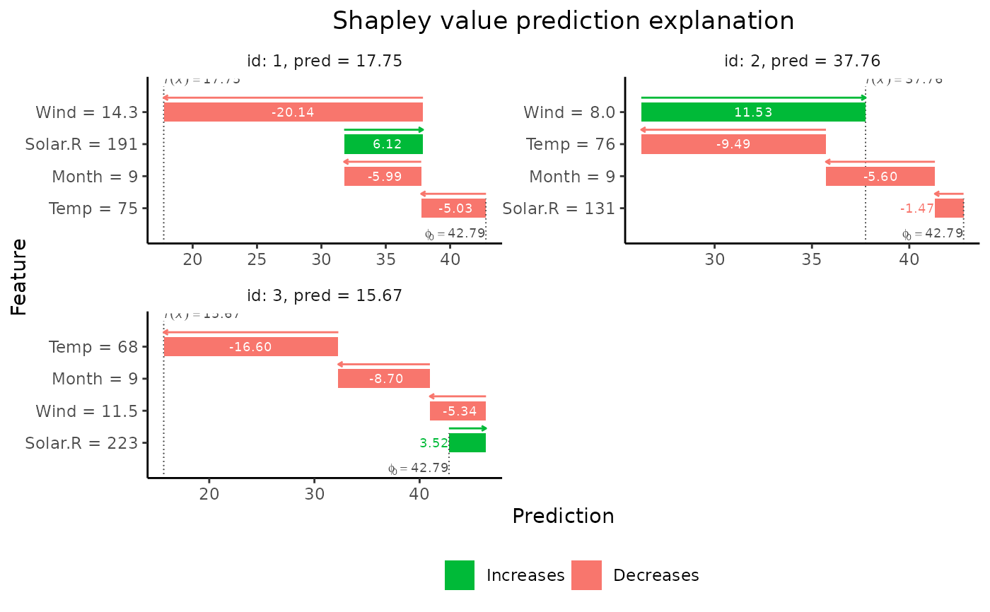
print(explain1$shapley_values_est)
#> explain_id none Solar.R Wind Temp Month
#> <int> <num> <num> <num> <num> <num>
#> 1: 1 42.78704 6.124296 -20.137653 -5.033967 -5.987303
#> 2: 2 42.78704 -1.470838 11.525868 -9.487924 -5.597657
#> 3: 3 42.78704 3.524599 -5.335059 -16.599988 -8.703929
# Plot the results
if (requireNamespace("ggplot2", quietly = TRUE)) {
plot(explain1)
plot(explain1, plot_type = "waterfall")
}
 # Group-wise explanations
group_list <- list(A = c("Temp", "Month"), B = c("Wind", "Solar.R"))
explain_groups <- explain(
model = model,
x_explain = x_explain,
x_train = x_train,
group = group_list,
approach = "empirical",
phi0 = p,
n_MC_samples = 1e2
)
#> Success with message:
#> max_n_coalitions is NULL or larger than or 2^n_groups = 4,
#> and is therefore set to 2^n_groups = 4.
#>
#> ── Starting `shapr::explain()` at 2024-12-19 12:11:23 ──────────────────────────
#> • Model class: <lm>
#> • Approach: empirical
#> • Iterative estimation: FALSE
#> • Number of group-wise Shapley values: 2
#> • Number of observations to explain: 3
#> • Computations (temporary) saved at: /tmp/Rtmpyp2Dru/shapr_obj_330e27f23a26.rds
#>
#> ── Main computation started ──
#>
#> ℹ Using 4 of 4 coalitions.
print(explain_groups$shapley_values_est)
#> explain_id none A B
#> <int> <num> <num> <num>
#> 1: 1 42.78704 -11.63856 -13.396062
#> 2: 2 42.78704 -10.36824 5.337683
#> 3: 3 42.78704 -25.79874 -1.315633
# Separate and surrogate regression approaches with linear regression models.
# More complex regression models can be used, and we can use CV to
# tune the hyperparameters of the regression models and preprocess
# the data before sending it to the model. See the regression vignette
# (Shapley value explanations using the regression paradigm) for more
# details about the `regression_separate` and `regression_surrogate` approaches.
explain_separate_lm <- explain(
model = model,
x_explain = x_explain,
x_train = x_train,
phi0 = p,
approach = "regression_separate",
regression.model = parsnip::linear_reg()
)
#> Success with message:
#> max_n_coalitions is NULL or larger than or 2^n_features = 16,
#> and is therefore set to 2^n_features = 16.
#>
#> ── Starting `shapr::explain()` at 2024-12-19 12:11:24 ──────────────────────────
#> • Model class: <lm>
#> • Approach: regression_separate
#> • Iterative estimation: FALSE
#> • Number of feature-wise Shapley values: 4
#> • Number of observations to explain: 3
#> • Computations (temporary) saved at: /tmp/Rtmpyp2Dru/shapr_obj_330e599dcbf0.rds
#>
#> ── Main computation started ──
#>
#> ℹ Using 16 of 16 coalitions.
explain_surrogate_lm <- explain(
model = model,
x_explain = x_explain,
x_train = x_train,
phi0 = p,
approach = "regression_surrogate",
regression.model = parsnip::linear_reg()
)
#> Success with message:
#> max_n_coalitions is NULL or larger than or 2^n_features = 16,
#> and is therefore set to 2^n_features = 16.
#>
#> ── Starting `shapr::explain()` at 2024-12-19 12:11:25 ──────────────────────────
#> • Model class: <lm>
#> • Approach: regression_surrogate
#> • Iterative estimation: FALSE
#> • Number of feature-wise Shapley values: 4
#> • Number of observations to explain: 3
#> • Computations (temporary) saved at: /tmp/Rtmpyp2Dru/shapr_obj_330e1bbc2789.rds
#>
#> ── Main computation started ──
#>
#> ℹ Using 16 of 16 coalitions.
## iterative estimation
# For illustration purposes only. By default not used for such small dimensions as here
# Gaussian approach
explain_iterative <- explain(
model = model,
x_explain = x_explain,
x_train = x_train,
approach = "gaussian",
phi0 = p,
n_MC_samples = 1e2,
iterative = TRUE,
iterative_args = list(initial_n_coalitions = 10)
)
#> Success with message:
#> max_n_coalitions is NULL or larger than or 2^n_features = 16,
#> and is therefore set to 2^n_features = 16.
#>
#> ── Starting `shapr::explain()` at 2024-12-19 12:11:25 ──────────────────────────
#> • Model class: <lm>
#> • Approach: gaussian
#> • Iterative estimation: TRUE
#> • Number of feature-wise Shapley values: 4
#> • Number of observations to explain: 3
#> • Computations (temporary) saved at: /tmp/Rtmpyp2Dru/shapr_obj_330e1fe8c4d4.rds
#>
#> ── iterative computation started ──
#>
#> ── Iteration 1 ─────────────────────────────────────────────────────────────────
#> ℹ Using 10 of 16 coalitions, 10 new.
#>
#> ── Iteration 2 ─────────────────────────────────────────────────────────────────
#> ℹ Using 12 of 16 coalitions, 2 new.
#>
#> ── Iteration 3 ─────────────────────────────────────────────────────────────────
#> ℹ Using 14 of 16 coalitions, 2 new.
# Group-wise explanations
group_list <- list(A = c("Temp", "Month"), B = c("Wind", "Solar.R"))
explain_groups <- explain(
model = model,
x_explain = x_explain,
x_train = x_train,
group = group_list,
approach = "empirical",
phi0 = p,
n_MC_samples = 1e2
)
#> Success with message:
#> max_n_coalitions is NULL or larger than or 2^n_groups = 4,
#> and is therefore set to 2^n_groups = 4.
#>
#> ── Starting `shapr::explain()` at 2024-12-19 12:11:23 ──────────────────────────
#> • Model class: <lm>
#> • Approach: empirical
#> • Iterative estimation: FALSE
#> • Number of group-wise Shapley values: 2
#> • Number of observations to explain: 3
#> • Computations (temporary) saved at: /tmp/Rtmpyp2Dru/shapr_obj_330e27f23a26.rds
#>
#> ── Main computation started ──
#>
#> ℹ Using 4 of 4 coalitions.
print(explain_groups$shapley_values_est)
#> explain_id none A B
#> <int> <num> <num> <num>
#> 1: 1 42.78704 -11.63856 -13.396062
#> 2: 2 42.78704 -10.36824 5.337683
#> 3: 3 42.78704 -25.79874 -1.315633
# Separate and surrogate regression approaches with linear regression models.
# More complex regression models can be used, and we can use CV to
# tune the hyperparameters of the regression models and preprocess
# the data before sending it to the model. See the regression vignette
# (Shapley value explanations using the regression paradigm) for more
# details about the `regression_separate` and `regression_surrogate` approaches.
explain_separate_lm <- explain(
model = model,
x_explain = x_explain,
x_train = x_train,
phi0 = p,
approach = "regression_separate",
regression.model = parsnip::linear_reg()
)
#> Success with message:
#> max_n_coalitions is NULL or larger than or 2^n_features = 16,
#> and is therefore set to 2^n_features = 16.
#>
#> ── Starting `shapr::explain()` at 2024-12-19 12:11:24 ──────────────────────────
#> • Model class: <lm>
#> • Approach: regression_separate
#> • Iterative estimation: FALSE
#> • Number of feature-wise Shapley values: 4
#> • Number of observations to explain: 3
#> • Computations (temporary) saved at: /tmp/Rtmpyp2Dru/shapr_obj_330e599dcbf0.rds
#>
#> ── Main computation started ──
#>
#> ℹ Using 16 of 16 coalitions.
explain_surrogate_lm <- explain(
model = model,
x_explain = x_explain,
x_train = x_train,
phi0 = p,
approach = "regression_surrogate",
regression.model = parsnip::linear_reg()
)
#> Success with message:
#> max_n_coalitions is NULL or larger than or 2^n_features = 16,
#> and is therefore set to 2^n_features = 16.
#>
#> ── Starting `shapr::explain()` at 2024-12-19 12:11:25 ──────────────────────────
#> • Model class: <lm>
#> • Approach: regression_surrogate
#> • Iterative estimation: FALSE
#> • Number of feature-wise Shapley values: 4
#> • Number of observations to explain: 3
#> • Computations (temporary) saved at: /tmp/Rtmpyp2Dru/shapr_obj_330e1bbc2789.rds
#>
#> ── Main computation started ──
#>
#> ℹ Using 16 of 16 coalitions.
## iterative estimation
# For illustration purposes only. By default not used for such small dimensions as here
# Gaussian approach
explain_iterative <- explain(
model = model,
x_explain = x_explain,
x_train = x_train,
approach = "gaussian",
phi0 = p,
n_MC_samples = 1e2,
iterative = TRUE,
iterative_args = list(initial_n_coalitions = 10)
)
#> Success with message:
#> max_n_coalitions is NULL or larger than or 2^n_features = 16,
#> and is therefore set to 2^n_features = 16.
#>
#> ── Starting `shapr::explain()` at 2024-12-19 12:11:25 ──────────────────────────
#> • Model class: <lm>
#> • Approach: gaussian
#> • Iterative estimation: TRUE
#> • Number of feature-wise Shapley values: 4
#> • Number of observations to explain: 3
#> • Computations (temporary) saved at: /tmp/Rtmpyp2Dru/shapr_obj_330e1fe8c4d4.rds
#>
#> ── iterative computation started ──
#>
#> ── Iteration 1 ─────────────────────────────────────────────────────────────────
#> ℹ Using 10 of 16 coalitions, 10 new.
#>
#> ── Iteration 2 ─────────────────────────────────────────────────────────────────
#> ℹ Using 12 of 16 coalitions, 2 new.
#>
#> ── Iteration 3 ─────────────────────────────────────────────────────────────────
#> ℹ Using 14 of 16 coalitions, 2 new.