Shapley value explanations using the regression paradigm
Lars Henry Berge Olsen
Source:vignettes/understanding_shapr_regression.Rmd
understanding_shapr_regression.RmdThis vignette elaborates and demonstrates the regression paradigm explained in Olsen et al. (2024). We describe how to specify the regression model, how to enable automatic cross-validation of the model’s hyperparameters, and applying pre-processing steps to the data before fitting the regression models. We refer to Olsen et al. (2024) for when one should use the different paradigms, method classes, and methods.
Olsen et al. (2024) divides the regression paradigm into the separate and surrogate regression method classes. In this vignette, we briefly introduce the two method classes. For an in-depth explanation, we refer the reader to Sections 3.5 and 3.6 in Olsen et al. (2024).
Briefly stated, the regression paradigm uses regression models to directly estimate the contribution function . The separate regression method class fits a separate regression model for each coalition , while the surrogate regression method class fits a single regression model to simultaneously predict the contribution function for all coalitions.
The shapr package supports any regression model from the
popular tidymodels package developed by Kuhn and Wickham (2020). The tidymodels framework
is a collection of packages for modeling and machine learning using tidyverse principles.
Some packages included in the tidymodels framework are
parsnip, recipes, workflows
tune, and rsample; see the setup section below for more examples. Furthermore,
click here to
access the complete list of supported regression models in the
tidymodels package. There are currently 80 supported
models, but the framework also allows adding regression models not
already implemented in tidymodels. It is also possible to
apply a wide range of pre-processing data steps. For instance, we can
either apply the linear regression model directly to the data or
pre-process the data to compute principal components (principal
component regression) before fitting the linear regression to the first
few eigenvectors (proessed features), see the pre-process section for an example. In the
add new regression methods section, we demonstrate
how to incorporate the projection pursuit regression model into the
tidymodels framework.
Note that our framework does not currently support model formulas
with special terms. For example, we do not support
parsnip::gen_additive_mod (i.e., mgcv::gam())
as it uses a non-standard notion in its formulas (in this case, the
s(feature, k = 2) function). See
?parsnip::model_formula() for more information. However,
this hurdle is overcome by pre-processing data steps containing spline
functions, which we showcase in the pre-process section for the separate
regression method class.
In the mixed data section, we demonstrate that the regression-based methods work on mixed data, too. However, we must add a pre-processing step for the regression models that do not natively support categorical data to encode the categorical features.
We use the same data and predictive models in this vignette as in the main vignette.
See the end of the continous data and mixed data sections for summary figures of all the methods used in this vignette to compute the Shapley value explanations.
The separate regression method class
In the regression_separate methods, we train a new
regression model
to estimate the conditional expectation for each coalition of
features.
The idea is to estimate separately for each coalition using regression. Let denote the training data, where is the th -dimensional input and is the associated response. For each coalition , the corresponding training data set is
For each data set , we train a regression model with respect to the mean squared error loss function. That is, we fit a regression model where the prediction is acting as the response and the feature subset of coalition , , is acting as the available features. The optimal model, with respect to the loss function, is , which corresponds to the contribution function . The regression model aims for the optimal, hence, it resembles/estimates the contribution function, i.e., .
Code
In this supplementary vignette, we use the same data and explain the
same model type as in the main vignette. We train a simple
xgboost model on the airquality dataset and
demonstrate how to use the shapr and the separate
regression method class to explain the individual predictions.
Setup
First, we set up the airquality dataset and train an
xgboost model, whose predictions we want to explain using
the Shapley value explanation framework. We import all packages in the
tidymodels framework in the code chunk below, but we could
have specified them directly, too. In this vignette, we use the
following packages in the tidymodels framework:
parsnip, recipes, workflows,
dials, hardhat, tibble,
rlang, and ggplot2. We include the
package::function() notation throughout this vignette to
indicate which package the functions originate from in the
tidymodels framework.
# Either use `library(tidymodels)` or separately specify the libraries indicated above
library(tidymodels)
library(shapr)

# Ensure that shapr's functions are prioritzed, otherwise we need to use the `shapr::`
# prefix when calling explain(). The `conflicted` package is imported by `tidymodels`.
conflicted::conflicts_prefer(shapr::explain, shapr::prepare_data)
# Other libraries
library(xgboost)
library(data.table)

data("airquality")
data <- data.table::as.data.table(airquality)
data <- data[complete.cases(data), ]

x_var <- c("Solar.R", "Wind", "Temp", "Month")
y_var <- "Ozone"

ind_x_explain <- 1:20
x_train <- data[-ind_x_explain, ..x_var]
y_train <- data[-ind_x_explain, get(y_var)]
x_explain <- data[ind_x_explain, ..x_var]

# Fitting a basic xgboost model to the training data
set.seed(123) # Set seed for reproducibility
model <- xgboost::xgboost(
  data = as.matrix(x_train),
  label = y_train,
  nround = 20,
  verbose = FALSE
)

# Specifying the phi_0, i.e. the expected prediction without any features
p0 <- mean(y_train)

# List to store all the explanation objects
explanation_list <- list()
To make the rest of the vignette easier to follow, we create some helper functions that plot and summarize the results of the explanation methods. This code block is optional to understand and can be skipped.
# Plot the MSEv criterion scores as horizontal bars and add dashed line of one method's score
plot_MSEv_scores <- function(explanation_list, method_line = NULL) {
  fig <- plot_MSEv_eval_crit(explanation_list) +
    ggplot2::theme(legend.position = "none") +
    ggplot2::coord_flip() +
    ggplot2::theme(plot.title = ggplot2::element_text(size = rel(0.95)))
  fig <- fig + ggplot2::scale_x_discrete(limits = rev(levels(fig$data$Method)))
  if (!is.null(method_line) && method_line %in% fig$data$Method) {
    fig <- fig + ggplot2::geom_hline(
      yintercept = fig$data$MSEv[fig$data$Method == method_line],
      linetype = "dashed",
      color = "black"
    )
  }
  return(fig)
}

# Extract the MSEv criterion scores and elapsed times
print_MSEv_scores_and_time <- function(explanation_list) {
  res <- as.data.frame(t(sapply(
    explanation_list,
    function(explanation) {
      round(c(explanation$MSEv$MSEv$MSEv, explanation$timing$total_time_secs), 2)
    }
  )))
  colnames(res) <- c("MSEv", "Time")
  return(res)
}

# Extract the k best methods in decreasing order
get_k_best_methods <- function(explanation_list, k_best) {
  res <- print_MSEv_scores_and_time(explanation_list)
  return(rownames(res)[order(res$MSEv)[seq(k_best)]])
}
To establish a baseline against which to compare the regression
methods, we will compare them with the Monte Carlo-based
empirical approach with default hyperparameters. In the
last section, we include all Monte Carlo-based methods implemented in
shapr to make an extensive comparison.
# Compute the Shapley value explanations using the empirical method
explanation_list$MC_empirical <- explain(
  model = model,
  x_explain = x_explain,
  x_train = x_train,
  approach = "empirical",
  phi0 = p0
)
#> Note: Feature classes extracted from the model contains NA.
#> Assuming feature classes from the data are correct.
#> Success with message:
#> max_n_coalitions is NULL or larger than or 2^n_features = 16,
#> and is therefore set to 2^n_features = 16.
#>
#> ── Starting `shapr::explain()` at 2024-11-21 13:43:36 ───────────────────────────────────────────────────────────────────────────────────────────────────────────────
#> • Model class: <xgb.Booster>
#> • Approach: empirical
#> • Iterative estimation: FALSE
#> • Number of feature-wise Shapley values: 4
#> • Number of observations to explain: 20
#> • Computations (temporary) saved at: '/tmp/RtmpgQii3E/shapr_obj_1aa7864f7b70f7.rds'
#>
#> ── Main computation started ──
#>
#> ℹ Using 16 of 16 coalitions.
Linear regression model
Then we compute the Shapley value explanations using a linear regression model and the separate regression method class.
explanation_list$sep_lm <- explain(
  model = model,
  x_explain = x_explain,
  x_train = x_train,
  phi0 = p0,
  approach = "regression_separate",
  regression.model = parsnip::linear_reg()
)
#> Note: Feature classes extracted from the model contains NA.
#> Assuming feature classes from the data are correct.
#> Success with message:
#> max_n_coalitions is NULL or larger than or 2^n_features = 16,
#> and is therefore set to 2^n_features = 16.
#>
#> ── Starting `shapr::explain()` at 2024-11-21 13:43:40 ───────────────────────────────────────────────────────────────────────────────────────────────────────────────
#> • Model class: <xgb.Booster>
#> • Approach: regression_separate
#> • Iterative estimation: FALSE
#> • Number of feature-wise Shapley values: 4
#> • Number of observations to explain: 20
#> • Computations (temporary) saved at: '/tmp/RtmpgQii3E/shapr_obj_1aa78629466589.rds'
#>
#> ── Main computation started ──
#>
#> ℹ Using 16 of 16 coalitions.
A linear model is often not flexible enough to properly model the
contribution function. Thus, it can produce inaccurate Shapley value
explanations. The figure below shows that the empirical
approach outperforms the linear regression model approach quite
significantly concerning the
evaluation criterion.
plot_MSEv_scores(explanation_list)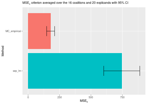
Pre-processing
This section describes how to pre-process the data before fitting the separate regression models. We demonstrate this for the linear regression model, but we can apply this pre-processing to other regression methods.
The recipe package in the tidymodels
framework contains many functions to pre-process the data before fitting
the model, for example, normalization, interaction, encodings, and
transformations (e.g., log, splines, pls, pca). Click here to
access a complete list of all available functions. The list also
contains functions for helping us select which features to apply the
functions to, e.g., recipes::all_predictors(),
recipes::all_numeric_predictors(), and
recipes::all_factor_predictors() apply the functions to all
features, only the numerical features, and only the factor features,
respectively. We can also specify the names of the features to which the
functions are applied. However, as the included features change in each
coalition, we need to check that the feature we want to apply the
function to is present in the dataset. We give an example of this
below.
First, we demonstrate how to compute the principal components and use (up to) the first two components for each separate linear regression model. We write “up to” as we can only compute a single principal component for the singleton coalitions, i.e., the feature itself. This regression model is called principal component regression.
explanation_list$sep_pcr <- explain(
  model = model,
  x_explain = x_explain,
  x_train = x_train,
  phi0 = p0,
  approach = "regression_separate",
  regression.model = parsnip::linear_reg(),
  regression.recipe_func = function(regression_recipe) {
    return(recipes::step_pca(regression_recipe, recipes::all_numeric_predictors(), num_comp = 2))
  }
)
#> Note: Feature classes extracted from the model contains NA.
#> Assuming feature classes from the data are correct.
#> Success with message:
#> max_n_coalitions is NULL or larger than or 2^n_features = 16,
#> and is therefore set to 2^n_features = 16.
#>
#> ── Starting `shapr::explain()` at 2024-11-21 13:43:41 ───────────────────────────────────────────────────────────────────────────────────────────────────────────────
#> • Model class: <xgb.Booster>
#> • Approach: regression_separate
#> • Iterative estimation: FALSE
#> • Number of feature-wise Shapley values: 4
#> • Number of observations to explain: 20
#> • Computations (temporary) saved at: '/tmp/RtmpgQii3E/shapr_obj_1aa78667333f80.rds'
#>
#> ── Main computation started ──
#>
#> ℹ Using 16 of 16 coalitions.
Second, we apply a pre-processing step that computes the basis expansions of the features using natural splines with two degrees of freedom. This is similar to fitting a generalized additive model.
explanation_list$sep_splines <- explain(
  model = model,
  x_explain = x_explain,
  x_train = x_train,
  phi0 = p0,
  approach = "regression_separate",
  regression.model = parsnip::linear_reg(),
  regression.recipe_func = function(regression_recipe) {
    return(recipes::step_ns(regression_recipe, recipes::all_numeric_predictors(), deg_free = 2))
  }
)
#> Note: Feature classes extracted from the model contains NA.
#> Assuming feature classes from the data are correct.
#> Success with message:
#> max_n_coalitions is NULL or larger than or 2^n_features = 16,
#> and is therefore set to 2^n_features = 16.
#>
#> ── Starting `shapr::explain()` at 2024-11-21 13:43:42 ───────────────────────────────────────────────────────────────────────────────────────────────────────────────
#> • Model class: <xgb.Booster>
#> • Approach: regression_separate
#> • Iterative estimation: FALSE
#> • Number of feature-wise Shapley values: 4
#> • Number of observations to explain: 20
#> • Computations (temporary) saved at: '/tmp/RtmpgQii3E/shapr_obj_1aa78652874079.rds'
#>
#> ── Main computation started ──
#>
#> ℹ Using 16 of 16 coalitions.
Finally, we provide an example where we include interactions between
the features Solar.R and Wind, log-transform
Solar.R, convert Wind to be between 0 and 1
and then take the square root, include polynomials of the third degree
for Temp, and apply the Box-Cox transformation to
Month. These transformations are only applied when the
features are present for the different separate models.
Furthermore, we stress that the purpose of this example is to highlight the framework’s flexibility, not that the transformations below are reasonable.
# Example function of how to apply step functions from the recipes package to specific features
regression.recipe_func <- function(recipe) {
  # Get the names of the present features
  feature_names <- recipe$var_info$variable[recipe$var_info$role == "predictor"]

  # If Solar.R and Wind is present, then we add the interaction between them
  if (all(c("Solar.R", "Wind") %in% feature_names)) {
    recipe <- recipes::step_interact(recipe, terms = ~ Solar.R:Wind)
  }

  # If Solar.R is present, then log transform it
  if ("Solar.R" %in% feature_names) recipe <- recipes::step_log(recipe, Solar.R)

  # If Wind is present, then scale it to be between 0 and 1 and then sqrt transform it
  if ("Wind" %in% feature_names) recipe <- recipes::step_sqrt(recipes::step_range(recipe, Wind))

  # If Temp is present, then expand it using orthogonal polynomials of degree 3
  if ("Temp" %in% feature_names) recipe <- recipes::step_poly(recipe, Temp, degree = 3)

  # If Month is present, then Box-Cox transform it
  if ("Month" %in% feature_names) recipe <- recipes::step_BoxCox(recipe, Month)

  # Finally we normalize all features (not needed as LM does this internally)
  recipe <- recipes::step_normalize(recipe, recipes::all_numeric_predictors())

  return(recipe)
}

# Compute the Shapley values using the pre-processing steps defined above
explanation_list$sep_reicpe_example <- explain(
  model = model,
  x_explain = x_explain,
  x_train = x_train,
  phi0 = p0,
  approach = "regression_separate",
  regression.model = parsnip::linear_reg(),
  regression.recipe_func = regression.recipe_func
)
#> Note: Feature classes extracted from the model contains NA.
#> Assuming feature classes from the data are correct.
#> Success with message:
#> max_n_coalitions is NULL or larger than or 2^n_features = 16,
#> and is therefore set to 2^n_features = 16.
#>
#> ── Starting `shapr::explain()` at 2024-11-21 13:43:43 ───────────────────────────────────────────────────────────────────────────────────────────────────────────────
#> • Model class: <xgb.Booster>
#> • Approach: regression_separate
#> • Iterative estimation: FALSE
#> • Number of feature-wise Shapley values: 4
#> • Number of observations to explain: 20
#> • Computations (temporary) saved at: '/tmp/RtmpgQii3E/shapr_obj_1aa7862f1e5e2d.rds'
#>
#> ── Main computation started ──
#>
#> ℹ Using 16 of 16 coalitions.
We can examine the evaluation scores, and we see that the method using natural splines significantly outperforms the other methods.
# Compare the MSEv criterion of the different explanation methods
plot_MSEv_scores(explanation_list, method_line = "MC_empirical")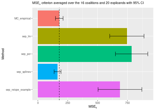
# Print the MSEv scores and the elapsed time (in seconds) for the different methods
print_MSEv_scores_and_time(explanation_list)
#>                      MSEv Time
#> MC_empirical       179.43 3.35
#> sep_lm             745.21 0.75
#> sep_pcr            784.91 0.88
#> sep_splines        165.13 0.89
#> sep_reicpe_example 687.45 1.25
Other regression models
In the following example, we use a decision tree model instead of the simple linear regression model.
The tidymodels framework supports several
implementations of the decision tree model. We use
set_engine("rpart") to specify that we want to use the
implementation in the rpart package, and we use
set_mode("regression") to specify that we are doing
regression. The tidymodels framework uses the default
hyperparameter values set in rpart when we do not specify
them. By searching for “decision tree” in the list of tidymodels,
we see that the default hyperparameter values for the decision_tree_rpart
model are tree_depth = 30, min_n = 2, and
cost_complexity = 0.01.
# Decision tree with specified parameters (stumps)
explanation_list$sep_tree_stump <- explain(
  model = model,
  x_explain = x_explain,
  x_train = x_train,
  phi0 = p0,
  approach = "regression_separate",
  regression.model = parsnip::decision_tree(
    tree_depth = 1,
    min_n = 2,
    cost_complexity = 0.01,
    engine = "rpart",
    mode = "regression"
  )
)
#> Note: Feature classes extracted from the model contains NA.
#> Assuming feature classes from the data are correct.
#> Success with message:
#> max_n_coalitions is NULL or larger than or 2^n_features = 16,
#> and is therefore set to 2^n_features = 16.
#>
#> ── Starting `shapr::explain()` at 2024-11-21 13:43:44 ───────────────────────────────────────────────────────────────────────────────────────────────────────────────
#> • Model class: <xgb.Booster>
#> • Approach: regression_separate
#> • Iterative estimation: FALSE
#> • Number of feature-wise Shapley values: 4
#> • Number of observations to explain: 20
#> • Computations (temporary) saved at: '/tmp/RtmpgQii3E/shapr_obj_1aa786b5a978d.rds'
#>
#> ── Main computation started ──
#>
#> ℹ Using 16 of 16 coalitions.

# Decision tree with default parameters
explanation_list$sep_tree_default <- explain(
  model = model,
  x_explain = x_explain,
  x_train = x_train,
  phi0 = p0,
  approach = "regression_separate",
  regression.model = parsnip::decision_tree(engine = "rpart", mode = "regression")
)
#> Note: Feature classes extracted from the model contains NA.
#> Assuming feature classes from the data are correct.
#> Success with message:
#> max_n_coalitions is NULL or larger than or 2^n_features = 16,
#> and is therefore set to 2^n_features = 16.
#>
#> ── Starting `shapr::explain()` at 2024-11-21 13:43:45 ───────────────────────────────────────────────────────────────────────────────────────────────────────────────
#> • Model class: <xgb.Booster>
#> • Approach: regression_separate
#> • Iterative estimation: FALSE
#> • Number of feature-wise Shapley values: 4
#> • Number of observations to explain: 20
#> • Computations (temporary) saved at: '/tmp/RtmpgQii3E/shapr_obj_1aa7867004239c.rds'
#>
#> ── Main computation started ──
#>
#> ℹ Using 16 of 16 coalitions.
We can also set
regression.model = parsnip::decision_tree(tree_depth = 1, min_n = 2, cost_complexity = 0.01) %>% parsnip::set_engine("rpart") %>% parsnip::set_mode("regression")
if we want to use the pipe function (%>%).
We can now compare the two new methods. The decision tree with default parameters outperforms the linear model approach concerning the criterion and is on the same level as the empirical approach. We obtained a worse method by using stumps, i.e., trees with depth one.
# Compare the MSEv criterion of the different explanation methods
plot_MSEv_scores(explanation_list, method_line = "MC_empirical")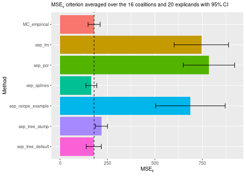
# Print the MSEv scores and the elapsed time (in seconds) for the different methods
print_MSEv_scores_and_time(explanation_list)
#>                      MSEv Time
#> MC_empirical       179.43 3.35
#> sep_lm             745.21 0.75
#> sep_pcr            784.91 0.88
#> sep_splines        165.13 0.89
#> sep_reicpe_example 687.45 1.25
#> sep_tree_stump     218.05 1.00
#> sep_tree_default   177.68 0.73
Cross-validation
Another option is to use cross-validation to tune the hyperparameters. To do this, we need to specify three things:
- In
regression.model, we need to specify which parameters to tune in the model. We do this by setting the parameter equal tohardhat::tune(). For example., if we want to tune thetree_depthparameter in theparsnip::decision_treemodel while using default parameters for the other parameters, then we setparsnip::decision_tree(tree_depth = hardhat::tune()). - In
regression.tune_values, we must provide either a data.frame (can also be a data.table or tibble) containing the possible hyperparameter values or a function that takes in the training data for each combination/coalition and outputs a data.frame containing the possible hyperparameter values. The latter allows us to use different hyperparameter values for different coalition sizes, which is essential if a hyperparameter’s domain changes with the coalition size. For example, see the example below where we want to tune themtryparameter inranger(random forest). The column names ofregression.tune_values(or the output if it is a function) must match the tuneable hyperparameters specified inregression.model. For the example above,regression.tune_valuesmust be a one-column data.frame with the column nametree_depth. We can either manually specify the hyperparameter values or use thedialspackage, e.g.,dials::grid_regular(dials::tree_depth(), levels = 5). Or it can be a function that outputs a data.frame on the same form. - Specifying the
regression.vfold_cv_paraparameter is optional. If used, thenregression.vfold_cv_paramust be a list specifying the parameters to send to the cross-validation functionrsample::vfold_cv(). Use?rsample::vfold_cvto see the default parameters. The names of the objects in theregression.vfold_cv_paralist must match the parameter names inrsample::vfold_cv(). For example, if we want 5-fold cross-validation, we setregression.vfold_cv_para = list(v = 5).
First, let us look at some ways to specify
regression.tune_values. Note that dials have
several other grid functions, e.g., dials::grid_random()
and dials::grid_latin_hypercube().
# Possible ways to define the `regression.tune_values` object.
# function(x) dials::grid_regular(dials::tree_depth(), levels = 4)
dials::grid_regular(dials::tree_depth(), levels = 4)
data.table(tree_depth = c(1, 5, 10, 15)) # Can also use data.frame or tibble

# For several features
# function(x) dials::grid_regular(dials::tree_depth(), dials::cost_complexity(), levels = 3)
dials::grid_regular(dials::tree_depth(), dials::cost_complexity(), levels = 3)
expand.grid(tree_depth = c(1, 3, 5), cost_complexity = c(0.001, 0.05, 0.01))
We will now demonstrate how to use cross-validation to fine-tune the
separate decision tree regression method. In the following examples, we
consider two versions. In the first example, we use cross-validation to
tune the tree_depth parameter using the
dials::grid_regular() function. In the second example, we
tune both the tree_depth and cost_complexity
parameters, but we will manually specify the possible hyperparameter
values this time.
# Decision tree with cross validated depth (default values other parameters)
explanation_list$sep_tree_cv <- explain(
  model = model,
  x_explain = x_explain,
  x_train = x_train,
  phi0 = p0,
  approach = "regression_separate",
  regression.model = parsnip::decision_tree(
    tree_depth = hardhat::tune(), engine = "rpart", mode = "regression"
  ),
  regression.tune_values = dials::grid_regular(dials::tree_depth(), levels = 4),
  regression.vfold_cv_para = list(v = 5)
)
#> Note: Feature classes extracted from the model contains NA.
#> Assuming feature classes from the data are correct.
#> Success with message:
#> max_n_coalitions is NULL or larger than or 2^n_features = 16,
#> and is therefore set to 2^n_features = 16.
#>
#> ── Starting `shapr::explain()` at 2024-11-21 13:43:46 ───────────────────────────────────────────────────────────────────────────────────────────────────────────────
#> • Model class: <xgb.Booster>
#> • Approach: regression_separate
#> • Iterative estimation: FALSE
#> • Number of feature-wise Shapley values: 4
#> • Number of observations to explain: 20
#> • Computations (temporary) saved at: '/tmp/RtmpgQii3E/shapr_obj_1aa7862e01b595.rds'
#>
#> ── Main computation started ──
#>
#> ℹ Using 16 of 16 coalitions.

# Use trees with cross-validation on the depth and cost complexity. Manually set the values.
explanation_list$sep_tree_cv_2 <- explain(
  model = model,
  x_explain = x_explain,
  x_train = x_train,
  phi0 = p0,
  approach = "regression_separate",
  regression.model = parsnip::decision_tree(
    tree_depth = hardhat::tune(),
    cost_complexity = hardhat::tune(),
    engine = "rpart",
    mode = "regression"
  ),
  regression.tune_values =
    expand.grid(tree_depth = c(1, 3, 5), cost_complexity = c(0.001, 0.01, 0.1)),
  regression.vfold_cv_para = list(v = 5)
)
#> Note: Feature classes extracted from the model contains NA.
#> Assuming feature classes from the data are correct.
#> Success with message:
#> max_n_coalitions is NULL or larger than or 2^n_features = 16,
#> and is therefore set to 2^n_features = 16.
#>
#> ── Starting `shapr::explain()` at 2024-11-21 13:43:59 ───────────────────────────────────────────────────────────────────────────────────────────────────────────────
#> • Model class: <xgb.Booster>
#> • Approach: regression_separate
#> • Iterative estimation: FALSE
#> • Number of feature-wise Shapley values: 4
#> • Number of observations to explain: 20
#> • Computations (temporary) saved at: '/tmp/RtmpgQii3E/shapr_obj_1aa78615cc7432.rds'
#>
#> ── Main computation started ──
#>
#> ℹ Using 16 of 16 coalitions.
We also include one example with a random forest model where the
tunable hyperparameter mtry depends on the coalition size.
Thus, regression.tune_values must be a function that
returns a data.frame where the hyperparameter values for
mtry will change based on the coalition size. If we do not
let regression.tune_values be a function, then
tidymodels will crash for any mtry higher than
1. Furthermore, by setting letting
"vS_details" %in% verbose, we receive get messages with the
results of the cross-validation procedure ran within shapr.
Note that the tested hyperparameter value combinations change based on
the coalition size.
# Using random forest with default parameters
explanation_list$sep_rf <- explain(
  model = model,
  x_explain = x_explain,
  x_train = x_train,
  phi0 = p0,
  approach = "regression_separate",
  regression.model = parsnip::rand_forest(engine = "ranger", mode = "regression")
)
#> Note: Feature classes extracted from the model contains NA.
#> Assuming feature classes from the data are correct.
#> Success with message:
#> max_n_coalitions is NULL or larger than or 2^n_features = 16,
#> and is therefore set to 2^n_features = 16.
#>
#> ── Starting `shapr::explain()` at 2024-11-21 13:44:24 ───────────────────────────────────────────────────────────────────────────────────────────────────────────────
#> • Model class: <xgb.Booster>
#> • Approach: regression_separate
#> • Iterative estimation: FALSE
#> • Number of feature-wise Shapley values: 4
#> • Number of observations to explain: 20
#> • Computations (temporary) saved at: '/tmp/RtmpgQii3E/shapr_obj_1aa7863390470d.rds'
#>
#> ── Main computation started ──
#>
#> ℹ Using 16 of 16 coalitions.

# Using random forest with parameters tuned by cross-validation
explanation_list$sep_rf_cv <- explain(
  model = model,
  x_explain = x_explain,
  x_train = x_train,
  phi0 = p0,
  verbose = c("basic","vS_details"), # To get printouts
  approach = "regression_separate",
  regression.model = parsnip::rand_forest(
    mtry = hardhat::tune(), trees = hardhat::tune(), engine = "ranger", mode = "regression"
  ),
  regression.tune_values =
    function(x) {
      dials::grid_regular(dials::mtry(c(1, ncol(x))), dials::trees(c(50, 750)), levels = 3)
    },
  regression.vfold_cv_para = list(v = 5)
)
#> Note: Feature classes extracted from the model contains NA.
#> Assuming feature classes from the data are correct.
#> Success with message:
#> max_n_coalitions is NULL or larger than or 2^n_features = 16,
#> and is therefore set to 2^n_features = 16.
#>
#> ── Starting `shapr::explain()` at 2024-11-21 13:44:26 ───────────────────────────────────────────────────────────────────────────────────────────────────────────────
#> • Model class: <xgb.Booster>
#> • Approach: regression_separate
#> • Iterative estimation: FALSE
#> • Number of feature-wise Shapley values: 4
#> • Number of observations to explain: 20
#> • Computations (temporary) saved at: '/tmp/RtmpgQii3E/shapr_obj_1aa7865f901637.rds'
#>
#> ── Additional details about the regression model
#> Random Forest Model Specification (regression)
#>
#> Main Arguments: mtry = hardhat::tune() trees = hardhat::tune()
#>
#> Computational engine: ranger
#>
#> ── Main computation started ──
#>
#> ℹ Using 16 of 16 coalitions.
#>
#> ── Extra info about the tuning of the regression model ──
#>
#> ── Top 6 best configs for  v(1 4) (using 5-fold CV)
#> #1: mtry = 1 trees = 50 rmse = 28.43 rmse_std_err = 3.02
#> #2: mtry = 1 trees = 750 rmse = 28.76 rmse_std_err = 2.57
#> #3: mtry = 1 trees = 400 rmse = 28.80 rmse_std_err = 2.64
#> #4: mtry = 2 trees = 50 rmse = 29.27 rmse_std_err = 2.29
#> #5: mtry = 2 trees = 400 rmse = 29.42 rmse_std_err = 2.40
#> #6: mtry = 2 trees = 750 rmse = 29.46 rmse_std_err = 2.20
#>
#> ── Top 6 best configs for  v(2 4) (using 5-fold CV)
#> #1: mtry = 1 trees = 50 rmse = 21.12 rmse_std_err = 0.73
#> #2: mtry = 1 trees = 750 rmse = 21.21 rmse_std_err = 0.66
#> #3: mtry = 2 trees = 400 rmse = 21.27 rmse_std_err = 1.02
#> #4: mtry = 2 trees = 750 rmse = 21.31 rmse_std_err = 1.01
#> #5: mtry = 1 trees = 400 rmse = 21.34 rmse_std_err = 0.69
#> #6: mtry = 2 trees = 50 rmse = 21.65 rmse_std_err = 0.94
#>
#> ── Top 6 best configs for  v(1 3) (using 5-fold CV)
#> #1: mtry = 1 trees = 50 rmse = 21.34 rmse_std_err = 3.18
#> #2: mtry = 1 trees = 400 rmse = 21.56 rmse_std_err = 3.13
#> #3: mtry = 1 trees = 750 rmse = 21.68 rmse_std_err = 3.13
#> #4: mtry = 2 trees = 50 rmse = 21.79 rmse_std_err = 3.10
#> #5: mtry = 2 trees = 750 rmse = 21.85 rmse_std_err = 2.98
#> #6: mtry = 2 trees = 400 rmse = 21.89 rmse_std_err = 2.97
#>
#> ── Top 6 best configs for  v(3 4) (using 5-fold CV)
#> #1: mtry = 1 trees = 750 rmse = 22.94 rmse_std_err = 4.33
#> #2: mtry = 1 trees = 400 rmse = 23.13 rmse_std_err = 4.23
#> #3: mtry = 1 trees = 50 rmse = 23.43 rmse_std_err = 4.13
#> #4: mtry = 2 trees = 400 rmse = 23.86 rmse_std_err = 3.77
#> #5: mtry = 2 trees = 750 rmse = 24.00 rmse_std_err = 3.78
#> #6: mtry = 2 trees = 50 rmse = 24.57 rmse_std_err = 4.08
#>
#> ── Top 6 best configs for  v(2 3) (using 5-fold CV)
#> #1: mtry = 2 trees = 50 rmse = 17.46 rmse_std_err = 2.26
#> #2: mtry = 2 trees = 750 rmse = 17.53 rmse_std_err = 2.43
#> #3: mtry = 2 trees = 400 rmse = 17.64 rmse_std_err = 2.38
#> #4: mtry = 1 trees = 750 rmse = 17.80 rmse_std_err = 2.09
#> #5: mtry = 1 trees = 50 rmse = 17.81 rmse_std_err = 1.79
#> #6: mtry = 1 trees = 400 rmse = 17.89 rmse_std_err = 2.13
#>
#> ── Top 3 best configs for  v(3) (using 5-fold CV)
#> #1: mtry = 1 trees = 50 rmse = 22.55 rmse_std_err = 4.68
#> #2: mtry = 1 trees = 400 rmse = 22.59 rmse_std_err = 4.63
#> #3: mtry = 1 trees = 750 rmse = 22.64 rmse_std_err = 4.65
#>
#> ── Top 6 best configs for  v(1 2) (using 5-fold CV)
#> #1: mtry = 1 trees = 400 rmse = 21.57 rmse_std_err = 2.25
#> #2: mtry = 1 trees = 750 rmse = 21.59 rmse_std_err = 2.29
#> #3: mtry = 1 trees = 50 rmse = 22.38 rmse_std_err = 2.10
#> #4: mtry = 2 trees = 400 rmse = 22.54 rmse_std_err = 2.09
#> #5: mtry = 2 trees = 750 rmse = 22.65 rmse_std_err = 2.09
#> #6: mtry = 2 trees = 50 rmse = 23.12 rmse_std_err = 2.23
#>
#> ── Top 3 best configs for  v(4) (using 5-fold CV)
#> #1: mtry = 1 trees = 750 rmse = 32.14 rmse_std_err = 4.32
#> #2: mtry = 1 trees = 400 rmse = 32.21 rmse_std_err = 4.31
#> #3: mtry = 1 trees = 50 rmse = 32.21 rmse_std_err = 4.25
#>
#> ── Top 3 best configs for  v(1) (using 5-fold CV)
#> #1: mtry = 1 trees = 50 rmse = 30.34 rmse_std_err = 3.40
#> #2: mtry = 1 trees = 750 rmse = 30.53 rmse_std_err = 3.31
#> #3: mtry = 1 trees = 400 rmse = 30.63 rmse_std_err = 3.32
#>
#> ── Top 3 best configs for  v(2) (using 5-fold CV)
#> #1: mtry = 1 trees = 750 rmse = 26.62 rmse_std_err = 2.33
#> #2: mtry = 1 trees = 400 rmse = 26.72 rmse_std_err = 2.29
#> #3: mtry = 1 trees = 50 rmse = 26.97 rmse_std_err = 2.24
#>
#> ── Top 9 best configs for  v(1 2 4) (using 5-fold CV)
#> #1: mtry = 2 trees = 750 rmse = 19.81 rmse_std_err = 1.53
#> #2: mtry = 2 trees = 400 rmse = 19.85 rmse_std_err = 1.64
#> #3: mtry = 1 trees = 750 rmse = 19.93 rmse_std_err = 1.93
#> #4: mtry = 1 trees = 400 rmse = 20.18 rmse_std_err = 1.90
#> #5: mtry = 2 trees = 50 rmse = 20.41 rmse_std_err = 1.56
#> #6: mtry = 3 trees = 50 rmse = 20.69 rmse_std_err = 1.54
#> #7: mtry = 3 trees = 750 rmse = 20.74 rmse_std_err = 1.69
#> #8: mtry = 3 trees = 400 rmse = 20.77 rmse_std_err = 1.76
#> #9: mtry = 1 trees = 50 rmse = 20.79 rmse_std_err = 1.89
#>
#> ── Top 9 best configs for  v(1 2 3) (using 5-fold CV)
#> #1: mtry = 2 trees = 400 rmse = 16.16 rmse_std_err = 2.75
#> #2: mtry = 3 trees = 400 rmse = 16.30 rmse_std_err = 2.80
#> #3: mtry = 2 trees = 750 rmse = 16.41 rmse_std_err = 2.79
#> #4: mtry = 3 trees = 750 rmse = 16.43 rmse_std_err = 2.82
#> #5: mtry = 3 trees = 50 rmse = 16.52 rmse_std_err = 2.52
#> #6: mtry = 1 trees = 750 rmse = 16.69 rmse_std_err = 3.15
#> #7: mtry = 2 trees = 50 rmse = 16.89 rmse_std_err = 2.76
#> #8: mtry = 1 trees = 400 rmse = 16.98 rmse_std_err = 2.93
#> #9: mtry = 1 trees = 50 rmse = 17.69 rmse_std_err = 3.16
#>
#> ── Top 9 best configs for  v(1 3 4) (using 5-fold CV)
#> #1: mtry = 1 trees = 400 rmse = 21.88 rmse_std_err = 4.33
#> #2: mtry = 1 trees = 750 rmse = 21.96 rmse_std_err = 4.38
#> #3: mtry = 1 trees = 50 rmse = 22.03 rmse_std_err = 4.07
#> #4: mtry = 2 trees = 400 rmse = 22.65 rmse_std_err = 4.11
#> #5: mtry = 2 trees = 750 rmse = 22.72 rmse_std_err = 4.09
#> #6: mtry = 2 trees = 50 rmse = 22.89 rmse_std_err = 3.97
#> #7: mtry = 3 trees = 400 rmse = 23.38 rmse_std_err = 3.80
#> #8: mtry = 3 trees = 750 rmse = 23.50 rmse_std_err = 3.77
#> #9: mtry = 3 trees = 50 rmse = 23.88 rmse_std_err = 3.64
#>
#> ── Top 9 best configs for  v(2 3 4) (using 5-fold CV)
#> #1: mtry = 3 trees = 50 rmse = 17.96 rmse_std_err = 1.34
#> #2: mtry = 1 trees = 50 rmse = 17.97 rmse_std_err = 2.40
#> #3: mtry = 1 trees = 750 rmse = 18.63 rmse_std_err = 1.99
#> #4: mtry = 2 trees = 400 rmse = 18.76 rmse_std_err = 1.42
#> #5: mtry = 1 trees = 400 rmse = 18.79 rmse_std_err = 2.14
#> #6: mtry = 2 trees = 750 rmse = 18.80 rmse_std_err = 1.49
#> #7: mtry = 3 trees = 750 rmse = 19.12 rmse_std_err = 1.68
#> #8: mtry = 3 trees = 400 rmse = 19.14 rmse_std_err = 1.65
#> #9: mtry = 2 trees = 50 rmse = 19.33 rmse_std_err = 1.67
We can look at the
evaluation criterion, and we see that cross-validation improves both the
decision tree and the random forest methods. The two cross-validated
decision tree methods are comparable, but the second version outperforms
the first version by a small margin. This comparison is somewhat unfair
for the empirical approach, which also has hyperparameters
we could potentially tune. However, shapr does not
currently provide a function to do this automatically. In the figure
below, we include a vertical line at the
score of the empirical method for easier comparison.
plot_MSEv_scores(explanation_list, method_line = "MC_empirical")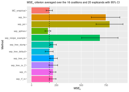
Furthermore, we must consider that cross-validation drastically increases the elapsed time (seconds) and determine if the increased precision is worth the extra computational time. We also see that the complex random forest method performs significantly worse than the simple decision tree method. This result indicates that even though we do hyperparameter tuning, we still overfit the data.
# Print the MSEv scores and the elapsed time (in seconds) for the different methods
print_MSEv_scores_and_time(explanation_list)
#>                      MSEv  Time
#> MC_empirical       179.43  3.35
#> sep_lm             745.21  0.75
#> sep_pcr            784.91  0.88
#> sep_splines        165.13  0.89
#> sep_reicpe_example 687.45  1.25
#> sep_tree_stump     218.05  1.00
#> sep_tree_default   177.68  0.73
#> sep_tree_cv        222.71 12.35
#> sep_tree_cv_2      219.45 25.59
#> sep_rf             217.00  1.23
#> sep_rf_cv          212.64 30.98
Parallelization
The future package can train the separate regression
models in parallel. More specifically, we parallelize both the training
step (when we fit the models) and the prediction step (when we compute
).
In the main vignette, we also explain how to enable progress bars.
In the code chunk below, we consider four regression-based methods.
The first method uses xgboost models with default
hyperparameter values, while the remaining three use cross-validation to
tune the number of trees. The second and third methods specify the same
potential hyperparameter values, but we run the former sequentially
while the latter is run in parallel to speed up the computations. The
fourth model is run in parallel but also tunes the depth of the trees
and not only the number of trees.
A small side note: If we let "vS_details" %in% verbose,
we can see which tree value shapr chooses for
each coalition. We would then see that the values 25, 50, 100, and 500
are never chosen. Thus, we can remove these values without influencing
the result and instead do a finer grid search among the lower values. We
do this in the fourth method.
# Regular xgboost with default parameters
explanation_list$sep_xgboost <- explain(
  model = model,
  x_explain = x_explain,
  x_train = x_train,
  phi0 = p0,
  approach = "regression_separate",
  regression.model = parsnip::boost_tree(engine = "xgboost", mode = "regression")
)
#> Note: Feature classes extracted from the model contains NA.
#> Assuming feature classes from the data are correct.
#> Success with message:
#> max_n_coalitions is NULL or larger than or 2^n_features = 16,
#> and is therefore set to 2^n_features = 16.
#>
#> ── Starting `shapr::explain()` at 2024-11-21 13:44:57 ───────────────────────────────────────────────────────────────────────────────────────────────────────────────
#> • Model class: <xgb.Booster>
#> • Approach: regression_separate
#> • Iterative estimation: FALSE
#> • Number of feature-wise Shapley values: 4
#> • Number of observations to explain: 20
#> • Computations (temporary) saved at: '/tmp/RtmpgQii3E/shapr_obj_1aa78636583f25.rds'
#>
#> ── Main computation started ──
#>
#> ℹ Using 16 of 16 coalitions.

# Cross validate the number of trees
explanation_list$sep_xgboost_cv <- explain(
  model = model,
  x_explain = x_explain,
  x_train = x_train,
  phi0 = p0,
  approach = "regression_separate",
  regression.model =
    parsnip::boost_tree(trees = hardhat::tune(), engine = "xgboost", mode = "regression"),
  regression.tune_values = expand.grid(trees = c(10, 15, 25, 50, 100, 500)),
  regression.vfold_cv_para = list(v = 5)
)
#> Note: Feature classes extracted from the model contains NA.
#> Assuming feature classes from the data are correct.
#> Success with message:
#> max_n_coalitions is NULL or larger than or 2^n_features = 16,
#> and is therefore set to 2^n_features = 16.
#>
#> ── Starting `shapr::explain()` at 2024-11-21 13:44:58 ───────────────────────────────────────────────────────────────────────────────────────────────────────────────
#> • Model class: <xgb.Booster>
#> • Approach: regression_separate
#> • Iterative estimation: FALSE
#> • Number of feature-wise Shapley values: 4
#> • Number of observations to explain: 20
#> • Computations (temporary) saved at: '/tmp/RtmpgQii3E/shapr_obj_1aa786931fb90.rds'
#>
#> ── Main computation started ──
#>
#> ℹ Using 16 of 16 coalitions.

# Cross validate the number of trees in parallel on two threads
future::plan(future::multisession, workers = 2)
explanation_list$sep_xgboost_cv_par <- explain(
  model = model,
  x_explain = x_explain,
  x_train = x_train,
  phi0 = p0,
  approach = "regression_separate",
  regression.model =
    parsnip::boost_tree(trees = hardhat::tune(), engine = "xgboost", mode = "regression"),
  regression.tune_values = expand.grid(trees = c(10, 15, 25, 50, 100, 500)),
  regression.vfold_cv_para = list(v = 5)
)
#> Note: Feature classes extracted from the model contains NA.
#> Assuming feature classes from the data are correct.
#> Success with message:
#> max_n_coalitions is NULL or larger than or 2^n_features = 16,
#> and is therefore set to 2^n_features = 16.
#>
#> ── Starting `shapr::explain()` at 2024-11-21 13:45:13 ───────────────────────────────────────────────────────────────────────────────────────────────────────────────
#> • Model class: <xgb.Booster>
#> • Approach: regression_separate
#> • Iterative estimation: FALSE
#> • Number of feature-wise Shapley values: 4
#> • Number of observations to explain: 20
#> • Computations (temporary) saved at: '/tmp/RtmpgQii3E/shapr_obj_1aa786491f190d.rds'
#>
#> ── Main computation started ──
#>
#> ℹ Using 16 of 16 coalitions.

# Use a finer grid of low values for `trees` and also tune `tree_depth`
future::plan(future::multisession, workers = 4) # Change to 4 threads due to more complex CV
explanation_list$sep_xgboost_cv_2_par <- explain(
  model = model,
  x_explain = x_explain,
  x_train = x_train,
  phi0 = p0,
  approach = "regression_separate",
  regression.model = parsnip::boost_tree(
    trees = hardhat::tune(),
    tree_depth = hardhat::tune(),
    engine = "xgboost",
    mode = "regression"
  ),
  regression.tune_values = expand.grid(trees = c(8, 10, 12, 15), tree_depth = c(4, 6, 8)),
  regression.vfold_cv_para = list(v = 5)
)
#> Note: Feature classes extracted from the model contains NA.
#> Assuming feature classes from the data are correct.
#> Success with message:
#> max_n_coalitions is NULL or larger than or 2^n_features = 16,
#> and is therefore set to 2^n_features = 16.
#>
#> ── Starting `shapr::explain()` at 2024-11-21 13:45:26 ───────────────────────────────────────────────────────────────────────────────────────────────────────────────
#> • Model class: <xgb.Booster>
#> • Approach: regression_separate
#> • Iterative estimation: FALSE
#> • Number of feature-wise Shapley values: 4
#> • Number of observations to explain: 20
#> • Computations (temporary) saved at: '/tmp/RtmpgQii3E/shapr_obj_1aa78652904b76.rds'
#>
#> ── Main computation started ──
#>
#> ℹ Using 16 of 16 coalitions.
future::plan(future::sequential) # To return to non-parallel computation
Looking at the elapsed time, we see that the parallel version with two workers is faster than the sequential version. Note that the elapsed time of the parallel version is not reduced by a factor of two as the creation of the parallel processes creates some additional overhead, which is significant in this small example. However, parallelization will yield considerable relative time improvements in more complex situations. E.g., in settings with (more) training observations with more features (i.e., more coalitions to compute) and situations with more time-consuming cross-validation (i.e., more folds, hyperparameters to tune, or hyperparameter values to consider). Furthermore, we see that conducting the cross-validation has lowered the criterion drastically. Finally, note that we obtain the same value whether we run the cross-validation in parallel or sequentially.
# Print the MSEv scores and the elapsed time (in seconds) for the different methods
print_MSEv_scores_and_time(explanation_list)
#>                        MSEv  Time
#> MC_empirical         179.43  3.35
#> sep_lm               745.21  0.75
#> sep_pcr              784.91  0.88
#> sep_splines          165.13  0.89
#> sep_reicpe_example   687.45  1.25
#> sep_tree_stump       218.05  1.00
#> sep_tree_default     177.68  0.73
#> sep_tree_cv          222.71 12.35
#> sep_tree_cv_2        219.45 25.59
#> sep_rf               217.00  1.23
#> sep_rf_cv            212.64 30.98
#> sep_xgboost          197.72  0.86
#> sep_xgboost_cv       169.83 14.60
#> sep_xgboost_cv_par   169.83 12.33
#> sep_xgboost_cv_2_par 153.13 13.99
The surrogate regression method class
Since the regression_separate methods train a new
regression model
for each coalition
,
a total of
models has to be trained, which can be time-consuming for slowly fitted
models. The minus two corresponds to the empty and grand coalitions.
The regression_surrogate method class builds on the
ideas from the regression_separate class, but instead of
fitting a new regression model for each coalition, we train a single
regression model
for all coalitions
(except the empty and grand coalitions), where
is an augmented version of
.
See Section 3.6.1 in Olsen et al. (2024)
for more details and examples.
We can also apply all the examples above for the separate regression method class to the surrogate regression method class.
Code
We demonstrate the surrogate method class using several regression
models below. More specifically, we use linear regression, random forest
(with and without (some) cross-validation), and xgboost
(with and without (some) cross-validation).
# Compute the Shapley value explanations using a surrogate linear regression model
explanation_list$sur_lm <- explain(
  model = model,
  x_explain = x_explain,
  x_train = x_train,
  phi0 = p0,
  approach = "regression_surrogate",
  regression.model = parsnip::linear_reg()
)
#> Note: Feature classes extracted from the model contains NA.
#> Assuming feature classes from the data are correct.
#> Success with message:
#> max_n_coalitions is NULL or larger than or 2^n_features = 16,
#> and is therefore set to 2^n_features = 16.
#>
#> ── Starting `shapr::explain()` at 2024-11-21 13:45:40 ───────────────────────────────────────────────────────────────────────────────────────────────────────────────
#> • Model class: <xgb.Booster>
#> • Approach: regression_surrogate
#> • Iterative estimation: FALSE
#> • Number of feature-wise Shapley values: 4
#> • Number of observations to explain: 20
#> • Computations (temporary) saved at: '/tmp/RtmpgQii3E/shapr_obj_1aa7867d8c7486.rds'
#>
#> ── Main computation started ──
#>
#> ℹ Using 16 of 16 coalitions.

# Using xgboost with default parameters as the surrogate model
explanation_list$sur_xgboost <- explain(
  model = model,
  x_explain = x_explain,
  x_train = x_train,
  phi0 = p0,
  approach = "regression_surrogate",
  regression.model = parsnip::boost_tree(engine = "xgboost", mode = "regression")
)
#> Note: Feature classes extracted from the model contains NA.
#> Assuming feature classes from the data are correct.
#> Success with message:
#> max_n_coalitions is NULL or larger than or 2^n_features = 16,
#> and is therefore set to 2^n_features = 16.
#>
#> ── Starting `shapr::explain()` at 2024-11-21 13:45:41 ───────────────────────────────────────────────────────────────────────────────────────────────────────────────
#> • Model class: <xgb.Booster>
#> • Approach: regression_surrogate
#> • Iterative estimation: FALSE
#> • Number of feature-wise Shapley values: 4
#> • Number of observations to explain: 20
#> • Computations (temporary) saved at: '/tmp/RtmpgQii3E/shapr_obj_1aa78660457178.rds'
#>
#> ── Main computation started ──
#>
#> ℹ Using 16 of 16 coalitions.

# Using xgboost with parameters tuned by cross-validation as the surrogate model
explanation_list$sur_xgboost_cv <- explain(
  model = model,
  x_explain = x_explain,
  x_train = x_train,
  phi0 = p0,
  approach = "regression_surrogate",
  regression.model = parsnip::boost_tree(
    trees = hardhat::tune(),
    tree_depth = hardhat::tune(),
    engine = "xgboost",
    mode = "regression"
  ),
  regression.tune_values = expand.grid(trees = c(5, 15, 25), tree_depth = c(2, 6, 10)),
  regression.vfold_cv_para = list(v = 5)
)
#> Note: Feature classes extracted from the model contains NA.
#> Assuming feature classes from the data are correct.
#> Success with message:
#> max_n_coalitions is NULL or larger than or 2^n_features = 16,
#> and is therefore set to 2^n_features = 16.
#>
#> ── Starting `shapr::explain()` at 2024-11-21 13:45:41 ───────────────────────────────────────────────────────────────────────────────────────────────────────────────
#> • Model class: <xgb.Booster>
#> • Approach: regression_surrogate
#> • Iterative estimation: FALSE
#> • Number of feature-wise Shapley values: 4
#> • Number of observations to explain: 20
#> • Computations (temporary) saved at: '/tmp/RtmpgQii3E/shapr_obj_1aa7865d9b9594.rds'
#>
#> ── Main computation started ──
#>
#> ℹ Using 16 of 16 coalitions.

# Using random forest with default parameters as the surrogate model
explanation_list$sur_rf <- explain(
  model = model,
  x_explain = x_explain,
  x_train = x_train,
  phi0 = p0,
  approach = "regression_surrogate",
  regression.model = parsnip::rand_forest(engine = "ranger", mode = "regression")
)
#> Note: Feature classes extracted from the model contains NA.
#> Assuming feature classes from the data are correct.
#> Success with message:
#> max_n_coalitions is NULL or larger than or 2^n_features = 16,
#> and is therefore set to 2^n_features = 16.
#>
#> ── Starting `shapr::explain()` at 2024-11-21 13:45:43 ───────────────────────────────────────────────────────────────────────────────────────────────────────────────
#> • Model class: <xgb.Booster>
#> • Approach: regression_surrogate
#> • Iterative estimation: FALSE
#> • Number of feature-wise Shapley values: 4
#> • Number of observations to explain: 20
#> • Computations (temporary) saved at: '/tmp/RtmpgQii3E/shapr_obj_1aa78658adae63.rds'
#>
#> ── Main computation started ──
#>
#> ℹ Using 16 of 16 coalitions.

# Using random forest with parameters tuned by cross-validation as the surrogate model
explanation_list$sur_rf_cv <- explain(
  model = model,
  x_explain = x_explain,
  x_train = x_train,
  phi0 = p0,
  approach = "regression_surrogate",
  regression.model = parsnip::rand_forest(
    mtry = hardhat::tune(), trees = hardhat::tune(), engine = "ranger", mode = "regression"
  ),
  regression.tune_values = dials::grid_regular(
    dials::mtry(c(1, ncol(x_explain))),
    dials::trees(c(50, 750)),
    levels = 6
  ),
  regression.vfold_cv_para = list(v = 5)
)
#> Note: Feature classes extracted from the model contains NA.
#> Assuming feature classes from the data are correct.
#> Success with message:
#> max_n_coalitions is NULL or larger than or 2^n_features = 16,
#> and is therefore set to 2^n_features = 16.
#>
#> ── Starting `shapr::explain()` at 2024-11-21 13:45:44 ───────────────────────────────────────────────────────────────────────────────────────────────────────────────
#> • Model class: <xgb.Booster>
#> • Approach: regression_surrogate
#> • Iterative estimation: FALSE
#> • Number of feature-wise Shapley values: 4
#> • Number of observations to explain: 20
#> • Computations (temporary) saved at: '/tmp/RtmpgQii3E/shapr_obj_1aa78642356367.rds'
#>
#> ── Main computation started ──
#>
#> ℹ Using 16 of 16 coalitions.
Parallelization
The code chunk below demonstrates how to run the surrogate regression
method class in parallel using the future package. The
setup procedure is identical to the one we specified for separate regression method class.
The training step of the surrogate regression model can be run in
parallel if we tune some of its hyperparameters. We parallelize the
cross-validation procedure in the training step; hence, we apply no
parallelization in the training step of a surrogate model with specified
hyperparameters. Furthermore, we parallelize the prediction step (when
we compute
)
in the same way as for the separate regression method class. Note that
parallelization will introduce some overhead, which can cause it to be
slower than running the code sequentially for smaller problems.
# Cross validate the number of trees in parallel on four threads
future::plan(future::multisession, workers = 4)
explanation_list$sur_rf_cv_par <- explain(
  model = model,
  x_explain = x_explain,
  x_train = x_train,
  phi0 = p0,
  approach = "regression_surrogate",
  regression.model = parsnip::rand_forest(
    mtry = hardhat::tune(), trees = hardhat::tune(), engine = "ranger", mode = "regression"
  ),
  regression.tune_values = dials::grid_regular(
    dials::mtry(c(1, ncol(x_explain))),
    dials::trees(c(50, 750)),
    levels = 6
  ),
  regression.vfold_cv_para = list(v = 5)
)
#> Note: Feature classes extracted from the model contains NA.
#> Assuming feature classes from the data are correct.
#> Success with message:
#> max_n_coalitions is NULL or larger than or 2^n_features = 16,
#> and is therefore set to 2^n_features = 16.
#>
#> ── Starting `shapr::explain()` at 2024-11-21 13:46:12 ───────────────────────────────────────────────────────────────────────────────────────────────────────────────
#> • Model class: <xgb.Booster>
#> • Approach: regression_surrogate
#> • Iterative estimation: FALSE
#> • Number of feature-wise Shapley values: 4
#> • Number of observations to explain: 20
#> • Computations (temporary) saved at: '/tmp/RtmpgQii3E/shapr_obj_1aa7866c6710c6.rds'
#>
#> ── Main computation started ──
#>
#> ℹ Using 16 of 16 coalitions.
future::plan(future::sequential) # To return to non-parallel computation

# Check that we get identical Shapley value explanations
all.equal(
  explanation_list$sur_rf_cv$shapley_values_est,
  explanation_list$sur_rf_cv_par$shapley_values_est
)
#> [1] TRUE
By looking at the
evaluation criterion and the elapsed time, we see that the surrogate
methods (except the linear regression model) outperform
empirical but are not on the same level as the best
separate regression methods. Furthermore, parallelization (4 cores)
decreased the elapsed time while obtaining the same
score. The identical scores mean that the separate models are identical
and independent of whether they were run sequentially or in
parallel.
# Print the MSEv scores and the elapsed time (in seconds) for the different methods
print_MSEv_scores_and_time(explanation_list)
#>                        MSEv  Time
#> MC_empirical         179.43  3.35
#> sep_lm               745.21  0.75
#> sep_pcr              784.91  0.88
#> sep_splines          165.13  0.89
#> sep_reicpe_example   687.45  1.25
#> sep_tree_stump       218.05  1.00
#> sep_tree_default     177.68  0.73
#> sep_tree_cv          222.71 12.35
#> sep_tree_cv_2        219.45 25.59
#> sep_rf               217.00  1.23
#> sep_rf_cv            212.64 30.98
#> sep_xgboost          197.72  0.86
#> sep_xgboost_cv       169.83 14.60
#> sep_xgboost_cv_par   169.83 12.33
#> sep_xgboost_cv_2_par 153.13 13.99
#> sur_lm               649.61  0.42
#> sur_xgboost          169.92  0.44
#> sur_xgboost_cv       169.87  2.01
#> sur_rf               201.23  0.69
#> sur_rf_cv            172.09 27.44
#> sur_rf_cv_par        172.09 20.81

# Compare the MSEv criterion of the different explanation methods.
# Include vertical line corresponding to the MSEv of the empirical method.
plot_MSEv_scores(explanation_list, method_line = "MC_empirical")
Add new regression methods
Even though the tidymodels framework contains many models, we might
want to add additional methods. In the following section, we demonstrate
how to add the projection pursuit regression (PPR) model as a new method
that can be used by shapr to compute the Shapley value
explanations, both as a separate and surrogate method.
We use the ppr() implementation in the
stats package to fit the PPR model. The model has several
hyperparameters that can be tuned, but the main hyperparameter is the
number of terms nterms. The following is based on the tidymodels
guide on adding new regression models. We refer to that guide for
more details and explanations of the code below.
# Step 1: register the model, modes, and arguments
parsnip::set_new_model(model = "ppr_reg")
parsnip::set_model_mode(model = "ppr_reg", mode = "regression")
parsnip::set_model_engine(model = "ppr_reg", mode = "regression", eng = "ppr")
parsnip::set_dependency("ppr_reg", eng = "ppr", pkg = "stats")

# If your function has several parameters, then we add one of these functions for each parameter
parsnip::set_model_arg(
  model = "ppr_reg",
  eng = "ppr",
  original = "nterms", # The original parameter name used in stats::ppr
  parsnip = "num_terms", # Change parameter name to match tidymodels' name convention
  func = list(pkg = "dials", fun = "num_terms"), # list(pkg = "stats", fun = "ppr"),
  has_submodel = FALSE
)

# Step 2: create the model function
ppr_reg <- function(mode = "regression", engine = "ppr", num_terms = NULL) {
  # Check for correct mode
  if (mode != "regression") rlang::abort("`mode` should be 'regression'")

  # Check for correct engine
  if (engine != "ppr") rlang::abort("`engine` should be 'ppr'")

  # Capture the arguments in quosures
  args <- list(num_terms = rlang::enquo(num_terms))

  # Save some empty slots for future parts of the specification
  parsnip::new_model_spec(
    "ppr_reg",
    args = args,
    eng_args = NULL,
    mode = mode,
    method = NULL,
    engine = engine
  )
}

# Step 3: add a fit module
parsnip::set_fit(
  model = "ppr_reg",
  eng = "ppr",
  mode = "regression",
  value = list(
    interface = "formula",
    protect = c("formula", "data", "weights"),
    func = c(pkg = "stats", fun = "ppr"),
    defaults = list()
  )
)

parsnip::set_encoding(
  model = "ppr_reg",
  eng = "ppr",
  mode = "regression",
  options = list(
    predictor_indicators = "traditional",
    compute_intercept = TRUE,
    remove_intercept = TRUE,
    allow_sparse_x = FALSE
  )
)

# Step 4: add modules for prediction
parsnip::set_pred(
  model = "ppr_reg",
  eng = "ppr",
  mode = "regression",
  type = "numeric",
  value = list(
    pre = NULL,
    post = NULL,
    func = c(fun = "predict"),
    args = list(
      object = quote(object$fit),
      newdata = quote(new_data),
      type = "numeric"
    )
  )
)

# Step 5: add tuning function (used by tune::tune_grid())
tunable.ppr_reg <- function(x, ...) {
  tibble::tibble(
    name = c("num_terms"),
    call_info = list(list(pkg = NULL, fun = "num_terms")),
    source = "model_spec",
    component = "ppr_reg",
    component_id = "main"
  )
}

# Step 6: add updating function (used by tune::finalize_workflow())
update.ppr_reg <- function(object, parameters = NULL, num_terms = NULL, ...) {
  rlang::check_installed("parsnip")
  eng_args <- parsnip::update_engine_parameters(object$eng_args, fresh = TRUE, ...)
  args <- list(num_terms = rlang::enquo(num_terms))
  args <- parsnip::update_main_parameters(args, parameters)
  parsnip::new_model_spec(
    "ppr_reg",
    args = args,
    eng_args = eng_args,
    mode = object$mode,
    method = NULL,
    engine = object$engine
  )
}
We can now use the PPR model to compute the Shapley value
explanations. We can use it as a separate and surrogate regression
method, and we can either set the number of terms num_terms
to a specific value or use cross-validation to tune the hyperparameter.
We do all four combinations below.
# PPR separate with specified number of terms
explanation_list$sep_ppr <- explain(
  model = model,
  x_explain = x_explain,
  x_train = x_train,
  phi0 = p0,
  approach = "regression_separate",
  regression.model = ppr_reg(num_terms = 2)
)
#> Note: Feature classes extracted from the model contains NA.
#> Assuming feature classes from the data are correct.
#> Success with message:
#> max_n_coalitions is NULL or larger than or 2^n_features = 16,
#> and is therefore set to 2^n_features = 16.
#>
#> ── Starting `shapr::explain()` at 2024-11-21 13:46:33 ───────────────────────────────────────────────────────────────────────────────────────────────────────────────
#> • Model class: <xgb.Booster>
#> • Approach: regression_separate
#> • Iterative estimation: FALSE
#> • Number of feature-wise Shapley values: 4
#> • Number of observations to explain: 20
#> • Computations (temporary) saved at: '/tmp/RtmpgQii3E/shapr_obj_1aa7863200c7e2.rds'
#>
#> ── Main computation started ──
#>
#> ℹ Using 16 of 16 coalitions.

# PPR separate with cross-validated number of terms
explanation_list$sep_ppr_cv <- explain(
  model = model,
  x_explain = x_explain,
  x_train = x_train,
  phi0 = p0,
  approach = "regression_separate",
  regression.model = ppr_reg(num_terms = hardhat::tune()),
  regression.tune_values = dials::grid_regular(dials::num_terms(c(1, 4)), levels = 3),
  regression.vfold_cv_para = list(v = 5)
)
#> Note: Feature classes extracted from the model contains NA.
#> Assuming feature classes from the data are correct.
#> Success with message:
#> max_n_coalitions is NULL or larger than or 2^n_features = 16,
#> and is therefore set to 2^n_features = 16.
#>
#> ── Starting `shapr::explain()` at 2024-11-21 13:46:34 ───────────────────────────────────────────────────────────────────────────────────────────────────────────────
#> • Model class: <xgb.Booster>
#> • Approach: regression_separate
#> • Iterative estimation: FALSE
#> • Number of feature-wise Shapley values: 4
#> • Number of observations to explain: 20
#> • Computations (temporary) saved at: '/tmp/RtmpgQii3E/shapr_obj_1aa7865e9cc51b.rds'
#>
#> ── Main computation started ──
#>
#> ℹ Using 16 of 16 coalitions.

# PPR surrogate with specified number of terms
explanation_list$sur_ppr <- explain(
  model = model,
  x_explain = x_explain,
  x_train = x_train,
  phi0 = p0,
  approach = "regression_surrogate",
  regression.model = ppr_reg(num_terms = 3)
)
#> Note: Feature classes extracted from the model contains NA.
#> Assuming feature classes from the data are correct.
#> Success with message:
#> max_n_coalitions is NULL or larger than or 2^n_features = 16,
#> and is therefore set to 2^n_features = 16.
#>
#> ── Starting `shapr::explain()` at 2024-11-21 13:46:44 ───────────────────────────────────────────────────────────────────────────────────────────────────────────────
#> • Model class: <xgb.Booster>
#> • Approach: regression_surrogate
#> • Iterative estimation: FALSE
#> • Number of feature-wise Shapley values: 4
#> • Number of observations to explain: 20
#> • Computations (temporary) saved at: '/tmp/RtmpgQii3E/shapr_obj_1aa786796408ed.rds'
#>
#> ── Main computation started ──
#>
#> ℹ Using 16 of 16 coalitions.

# PPR surrogate with cross-validated number of terms
explanation_list$sur_ppr_cv <- explain(
  model = model,
  x_explain = x_explain,
  x_train = x_train,
  phi0 = p0,
  approach = "regression_surrogate",
  regression.model = ppr_reg(num_terms = hardhat::tune()),
  regression.tune_values = dials::grid_regular(dials::num_terms(c(1, 8)), levels = 4),
  regression.vfold_cv_para = list(v = 5)
)
#> Note: Feature classes extracted from the model contains NA.
#> Assuming feature classes from the data are correct.
#> Success with message:
#> max_n_coalitions is NULL or larger than or 2^n_features = 16,
#> and is therefore set to 2^n_features = 16.
#>
#> ── Starting `shapr::explain()` at 2024-11-21 13:46:45 ───────────────────────────────────────────────────────────────────────────────────────────────────────────────
#> • Model class: <xgb.Booster>
#> • Approach: regression_surrogate
#> • Iterative estimation: FALSE
#> • Number of feature-wise Shapley values: 4
#> • Number of observations to explain: 20
#> • Computations (temporary) saved at: '/tmp/RtmpgQii3E/shapr_obj_1aa7863ebffc8.rds'
#>
#> ── Main computation started ──
#>
#> ℹ Using 16 of 16 coalitions.
We can then compare the and some of the Shapley value explanations. We see that conducting cross-validation improves the evaluation criterion, but also increase the running time.
# Print the MSEv scores and the elapsed time (in seconds) for the different methods
print_MSEv_scores_and_time(explanation_list)
#>                        MSEv  Time
#> MC_empirical         179.43  3.35
#> sep_lm               745.21  0.75
#> sep_pcr              784.91  0.88
#> sep_splines          165.13  0.89
#> sep_reicpe_example   687.45  1.25
#> sep_tree_stump       218.05  1.00
#> sep_tree_default     177.68  0.73
#> sep_tree_cv          222.71 12.35
#> sep_tree_cv_2        219.45 25.59
#> sep_rf               217.00  1.23
#> sep_rf_cv            212.64 30.98
#> sep_xgboost          197.72  0.86
#> sep_xgboost_cv       169.83 14.60
#> sep_xgboost_cv_par   169.83 12.33
#> sep_xgboost_cv_2_par 153.13 13.99
#> sur_lm               649.61  0.42
#> sur_xgboost          169.92  0.44
#> sur_xgboost_cv       169.87  2.01
#> sur_rf               201.23  0.69
#> sur_rf_cv            172.09 27.44
#> sur_rf_cv_par        172.09 20.81
#> sep_ppr              327.23  0.76
#> sep_ppr_cv           246.28 10.24
#> sur_ppr              395.42  0.39
#> sur_ppr_cv           415.62  1.57

# Compare the MSEv criterion of the different explanation methods
plot_MSEv_scores(explanation_list, method_line = "MC_empirical")
Summary figures
In this section, we compute the Shapley value explanations for the
Monte Carlo-based methods in the shapr package and compare
the results with all the regression-based methods above. The purpose of
this vignette is to demonstrate the rich possibilities that the
regression paradigm and the tidymodels framework adds to
the shapr package.
In the code chunk below, we compute the Shapley value explanations using the different Monte Carlo-based methods.
explanation_list_MC <- list()

# Compute the Shapley value explanations using the independence method
explanation_list_MC$MC_independence <- explain(
  model = model,
  x_explain = x_explain,
  x_train = x_train,
  approach = "independence",
  phi0 = p0
)
#> Note: Feature classes extracted from the model contains NA.
#> Assuming feature classes from the data are correct.
#> Success with message:
#> max_n_coalitions is NULL or larger than or 2^n_features = 16,
#> and is therefore set to 2^n_features = 16.
#>
#> ── Starting `shapr::explain()` at 2024-11-21 13:46:47 ───────────────────────────────────────────────────────────────────────────────────────────────────────────────
#> • Model class: <xgb.Booster>
#> • Approach: independence
#> • Iterative estimation: FALSE
#> • Number of feature-wise Shapley values: 4
#> • Number of observations to explain: 20
#> • Computations (temporary) saved at: '/tmp/RtmpgQii3E/shapr_obj_1aa7862f2f3856.rds'
#>
#> ── Main computation started ──
#>
#> ℹ Using 16 of 16 coalitions.

# Copy the Shapley value explanations for the empirical method
explanation_list_MC$MC_empirical <- explanation_list$MC_empirical

# Compute the Shapley value explanations using the gaussian method
explanation_list_MC$MC_gaussian <- explain(
  model = model,
  x_explain = x_explain,
  x_train = x_train,
  approach = "gaussian",
  phi0 = p0
)
#> Note: Feature classes extracted from the model contains NA.
#> Assuming feature classes from the data are correct.
#> Success with message:
#> max_n_coalitions is NULL or larger than or 2^n_features = 16,
#> and is therefore set to 2^n_features = 16.
#>
#> ── Starting `shapr::explain()` at 2024-11-21 13:46:48 ───────────────────────────────────────────────────────────────────────────────────────────────────────────────
#> • Model class: <xgb.Booster>
#> • Approach: gaussian
#> • Iterative estimation: FALSE
#> • Number of feature-wise Shapley values: 4
#> • Number of observations to explain: 20
#> • Computations (temporary) saved at: '/tmp/RtmpgQii3E/shapr_obj_1aa78626579ea5.rds'
#>
#> ── Main computation started ──
#>
#> ℹ Using 16 of 16 coalitions.

# Compute the Shapley value explanations using the copula method
explanation_list_MC$MC_copula <- explain(
  model = model,
  x_explain = x_explain,
  x_train = x_train,
  approach = "copula",
  phi0 = p0
)
#> Note: Feature classes extracted from the model contains NA.
#> Assuming feature classes from the data are correct.
#> Success with message:
#> max_n_coalitions is NULL or larger than or 2^n_features = 16,
#> and is therefore set to 2^n_features = 16.
#>
#> ── Starting `shapr::explain()` at 2024-11-21 13:46:48 ───────────────────────────────────────────────────────────────────────────────────────────────────────────────
#> • Model class: <xgb.Booster>
#> • Approach: copula
#> • Iterative estimation: FALSE
#> • Number of feature-wise Shapley values: 4
#> • Number of observations to explain: 20
#> • Computations (temporary) saved at: '/tmp/RtmpgQii3E/shapr_obj_1aa78623a24f70.rds'
#>
#> ── Main computation started ──
#>
#> ℹ Using 16 of 16 coalitions.

# Compute the Shapley value explanations using the ctree method
explanation_list_MC$MC_ctree <- explain(
  model = model,
  x_explain = x_explain,
  x_train = x_train,
  approach = "ctree",
  phi0 = p0
)
#> Note: Feature classes extracted from the model contains NA.
#> Assuming feature classes from the data are correct.
#> Success with message:
#> max_n_coalitions is NULL or larger than or 2^n_features = 16,
#> and is therefore set to 2^n_features = 16.
#>
#> ── Starting `shapr::explain()` at 2024-11-21 13:46:49 ───────────────────────────────────────────────────────────────────────────────────────────────────────────────
#> • Model class: <xgb.Booster>
#> • Approach: ctree
#> • Iterative estimation: FALSE
#> • Number of feature-wise Shapley values: 4
#> • Number of observations to explain: 20
#> • Computations (temporary) saved at: '/tmp/RtmpgQii3E/shapr_obj_1aa78622c601b8.rds'
#>
#> ── Main computation started ──
#>
#> ℹ Using 16 of 16 coalitions.

# Compute the Shapley value explanations using the vaeac method
explanation_list_MC$MC_vaeac <- explain(
  model = model,
  x_explain = x_explain,
  x_train = x_train,
  approach = "vaeac",
  phi0 = p0,
  vaeac.epochs = 10
)
#> Note: Feature classes extracted from the model contains NA.
#> Assuming feature classes from the data are correct.
#> Success with message:
#> max_n_coalitions is NULL or larger than or 2^n_features = 16,
#> and is therefore set to 2^n_features = 16.
#>
#> ── Starting `shapr::explain()` at 2024-11-21 13:46:50 ───────────────────────────────────────────────────────────────────────────────────────────────────────────────
#> • Model class: <xgb.Booster>
#> • Approach: vaeac
#> • Iterative estimation: FALSE
#> • Number of feature-wise Shapley values: 4
#> • Number of observations to explain: 20
#> • Computations (temporary) saved at: '/tmp/RtmpgQii3E/shapr_obj_1aa7863c7421dd.rds'
#>
#> ── Main computation started ──
#>
#> ℹ Using 16 of 16 coalitions.

# Combine the two explanations lists
explanation_list$MC_empirical <- NULL
explanation_list <- c(explanation_list_MC, explanation_list)
We then compare the compare the regression and Monte Carlo-based
methods by plotting the
evaluation criterion. We continue with include a vertical line
corresponding to the
of the MC_empirical method to make the comparison
easier.
# Print the MSEv scores and the elapsed time (in seconds) for the different methods
print_MSEv_scores_and_time(explanation_list)
#>                        MSEv   Time
#> MC_independence      206.92   0.63
#> MC_empirical         179.43   3.35
#> MC_gaussian          235.15   0.47
#> MC_copula            237.35   0.53
#> MC_ctree             190.82   1.90
#> MC_vaeac             145.06 125.93
#> sep_lm               745.21   0.75
#> sep_pcr              784.91   0.88
#> sep_splines          165.13   0.89
#> sep_reicpe_example   687.45   1.25
#> sep_tree_stump       218.05   1.00
#> sep_tree_default     177.68   0.73
#> sep_tree_cv          222.71  12.35
#> sep_tree_cv_2        219.45  25.59
#> sep_rf               217.00   1.23
#> sep_rf_cv            212.64  30.98
#> sep_xgboost          197.72   0.86
#> sep_xgboost_cv       169.83  14.60
#> sep_xgboost_cv_par   169.83  12.33
#> sep_xgboost_cv_2_par 153.13  13.99
#> sur_lm               649.61   0.42
#> sur_xgboost          169.92   0.44
#> sur_xgboost_cv       169.87   2.01
#> sur_rf               201.23   0.69
#> sur_rf_cv            172.09  27.44
#> sur_rf_cv_par        172.09  20.81
#> sep_ppr              327.23   0.76
#> sep_ppr_cv           246.28  10.24
#> sur_ppr              395.42   0.39
#> sur_ppr_cv           415.62   1.57

# Compare the MSEv criterion of the different explanation methods
# Include vertical line corresponding to the MSEv of the MC_empirical method
plot_MSEv_scores(explanation_list, method_line = "MC_empirical")
The vaeac approach is the best-performing method
according to the
evaluation criterion, while the sep_xgboost_cv_2_par is the
best-performing regression-based method. However, we should note that
the vaeac method is much slower and that the difference
between the
values is minuscule and inside the confidence intervals.
We can also order the methods to more easily look at the order of the methods according to the criterion.
order <- get_k_best_methods(explanation_list, k = length(explanation_list))
plot_MSEv_scores(explanation_list[order], method_line = "MC_empirical")
We can also examine the different Shapley value explanations for the first six explicands (two at a time), and we still sort the methods from best to worst. Most methods agree in the general directions, especially for the most important features (the features with the largest absolute Shapley values), but there are some differences for the less important features. These tendencies/discrepancies are often more visible for the methods with poor/larger values.
plot_SV_several_approaches(explanation_list[order], index_explicands = c(1, 2), facet_ncol = 1)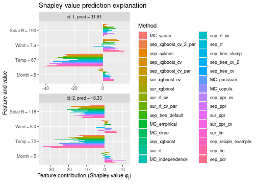
plot_SV_several_approaches(explanation_list[order], index_explicands = c(3, 4), facet_ncol = 1)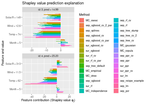
plot_SV_several_approaches(explanation_list[order], index_explicands = c(5, 6), facet_ncol = 1)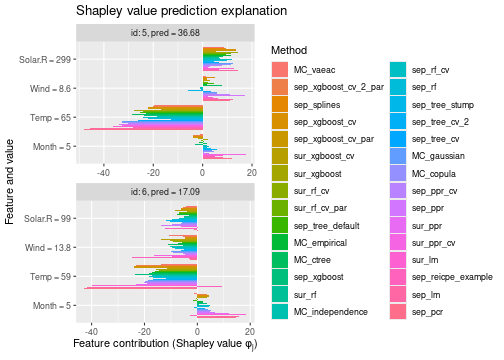
Here, we focus on the five best methods (and
MC_empricial) to make it easier to analyze the individual
Shapley value explanations, and we see a quite strong agreement between
the different methods.
# Extract the 5 best methods (and empirical)
best_methods <- get_k_best_methods(explanation_list, k = 5)
if (!"MC_empirical" %in% best_methods) best_methods <- c(best_methods, "MC_empirical")
plot_SV_several_approaches(explanation_list[best_methods], index_explicands = 1:4)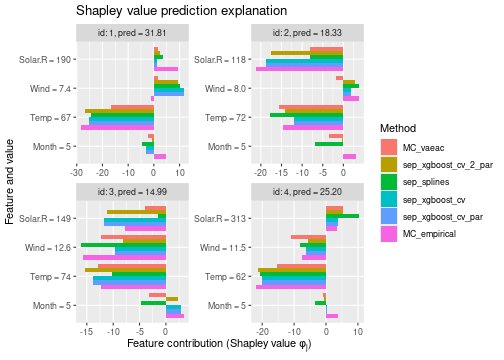
Mixed data
In this section, we replicate and extend the mixed data example from
the main vignette by demonstrating the separate and surrogate regression
methods. Of the Monte Carlo-based methods, only the
independence (not recommended), ctree, and
vaeac methods support mixed data. We can divide the
regression models into two groups based on whether the model can handle
categorical features by default or if we need to apply pre-processing of
the categorical features. By pre-processing, we mean that we need to
convert the categorical features into numerical values using, for
example, dummy features. We demonstrate this below using the
regression.recipe_func function.
Mixed data: setup
First, we copy the setup from the main vignette.
# convert the month variable to a factor
data_cat <- copy(data)[, Month_factor := as.factor(Month)]

data_train_cat <- data_cat[-ind_x_explain, ]
data_explain_cat <- data_cat[ind_x_explain, ]

x_var_cat <- c("Solar.R", "Wind", "Temp", "Month_factor")

x_train_cat <- data_train_cat[, ..x_var_cat]
x_explain_cat <- data_explain_cat[, ..x_var_cat]

p0_cat <- mean(y_train)

# Fitting an lm model here as xgboost does not handle categorical features directly
formula <- as.formula(paste0(y_var, " ~ ", paste0(x_var_cat, collapse = " + ")))
model_cat <- lm(formula, data_train_cat)

# We could also consider other models such as random forest which supports mixed data
# model_cat <- ranger(formula, data_train_cat)

# List to store the explanations for this mixed data setup
explanation_list_mixed <- list()
Mixed data: Monte Carlo-based methods
Second, we compute the explanations using the Monte Carlo-based methods.
explanation_list_mixed$MC_independence <- explain(
  model = model_cat,
  x_explain = x_explain_cat,
  x_train = x_train_cat,
  phi0 = p0_cat,
  approach = "independence"
)
#> Success with message:
#> max_n_coalitions is NULL or larger than or 2^n_features = 16,
#> and is therefore set to 2^n_features = 16.
#>
#> ── Starting `shapr::explain()` at 2024-11-21 13:49:00 ───────────────────────────────────────────────────────────────────────────────────────────────────────────────
#> • Model class: <lm>
#> • Approach: independence
#> • Iterative estimation: FALSE
#> • Number of feature-wise Shapley values: 4
#> • Number of observations to explain: 20
#> • Computations (temporary) saved at: '/tmp/RtmpgQii3E/shapr_obj_1aa786590644b4.rds'
#>
#> ── Main computation started ──
#>
#> ℹ Using 16 of 16 coalitions.

explanation_list_mixed$MC_ctree <- explain(
  model = model_cat,
  x_explain = x_explain_cat,
  x_train = x_train_cat,
  phi0 = p0_cat,
  approach = "ctree"
)
#> Success with message:
#> max_n_coalitions is NULL or larger than or 2^n_features = 16,
#> and is therefore set to 2^n_features = 16.
#>
#> ── Starting `shapr::explain()` at 2024-11-21 13:49:01 ───────────────────────────────────────────────────────────────────────────────────────────────────────────────
#> • Model class: <lm>
#> • Approach: ctree
#> • Iterative estimation: FALSE
#> • Number of feature-wise Shapley values: 4
#> • Number of observations to explain: 20
#> • Computations (temporary) saved at: '/tmp/RtmpgQii3E/shapr_obj_1aa786424cf108.rds'
#>
#> ── Main computation started ──
#>
#> ℹ Using 16 of 16 coalitions.

explanation_list_mixed$MC_vaeac <- explain(
  model = model_cat,
  x_explain = x_explain_cat,
  x_train = x_train_cat,
  phi0 = p0_cat,
  approach = "vaeac"
)
#> Success with message:
#> max_n_coalitions is NULL or larger than or 2^n_features = 16,
#> and is therefore set to 2^n_features = 16.
#>
#> ── Starting `shapr::explain()` at 2024-11-21 13:49:03 ───────────────────────────────────────────────────────────────────────────────────────────────────────────────
#> • Model class: <lm>
#> • Approach: vaeac
#> • Iterative estimation: FALSE
#> • Number of feature-wise Shapley values: 4
#> • Number of observations to explain: 20
#> • Computations (temporary) saved at: '/tmp/RtmpgQii3E/shapr_obj_1aa7865c8607f1.rds'
#>
#> ── Main computation started ──
#>
#> ℹ Using 16 of 16 coalitions.
Mixed data: separate regression methods
Third, we compute the Shapley value explanations using separate regression methods. We use many of the same regression models as we did above for the continuous data examples.
# Standard linear regression
explanation_list_mixed$sep_lm <- explain(
  model = model_cat,
  x_explain = x_explain_cat,
  x_train = x_train_cat,
  phi0 = p0_cat,
  approach = "regression_separate",
  regression.model = parsnip::linear_reg()
)
#> Success with message:
#> max_n_coalitions is NULL or larger than or 2^n_features = 16,
#> and is therefore set to 2^n_features = 16.
#>
#> ── Starting `shapr::explain()` at 2024-11-21 13:52:26 ───────────────────────────────────────────────────────────────────────────────────────────────────────────────
#> • Model class: <lm>
#> • Approach: regression_separate
#> • Iterative estimation: FALSE
#> • Number of feature-wise Shapley values: 4
#> • Number of observations to explain: 20
#> • Computations (temporary) saved at: '/tmp/RtmpgQii3E/shapr_obj_1aa7865611779c.rds'
#>
#> ── Main computation started ──
#>
#> ℹ Using 16 of 16 coalitions.

# Linear regression where we have added splines to the numerical features
explanation_list_mixed$sep_splines <- explain(
  model = model_cat,
  x_explain = x_explain_cat,
  x_train = x_train_cat,
  phi0 = p0_cat,
  approach = "regression_separate",
  regression.model = parsnip::linear_reg(),
  regression.recipe_func = function(regression_recipe) {
    return(step_ns(regression_recipe, all_numeric_predictors(), deg_free = 2))
  }
)
#> Success with message:
#> max_n_coalitions is NULL or larger than or 2^n_features = 16,
#> and is therefore set to 2^n_features = 16.
#>
#> ── Starting `shapr::explain()` at 2024-11-21 13:52:27 ───────────────────────────────────────────────────────────────────────────────────────────────────────────────
#> • Model class: <lm>
#> • Approach: regression_separate
#> • Iterative estimation: FALSE
#> • Number of feature-wise Shapley values: 4
#> • Number of observations to explain: 20
#> • Computations (temporary) saved at: '/tmp/RtmpgQii3E/shapr_obj_1aa78640377130.rds'
#>
#> ── Main computation started ──
#>
#> ℹ Using 16 of 16 coalitions.

# Decision tree with default parameters
explanation_list_mixed$sep_tree <- explain(
  model = model_cat,
  x_explain = x_explain_cat,
  x_train = x_train_cat,
  phi0 = p0_cat,
  approach = "regression_separate",
  regression.model = parsnip::decision_tree(engine = "rpart", mode = "regression")
)
#> Success with message:
#> max_n_coalitions is NULL or larger than or 2^n_features = 16,
#> and is therefore set to 2^n_features = 16.
#>
#> ── Starting `shapr::explain()` at 2024-11-21 13:52:28 ───────────────────────────────────────────────────────────────────────────────────────────────────────────────
#> • Model class: <lm>
#> • Approach: regression_separate
#> • Iterative estimation: FALSE
#> • Number of feature-wise Shapley values: 4
#> • Number of observations to explain: 20
#> • Computations (temporary) saved at: '/tmp/RtmpgQii3E/shapr_obj_1aa7864f9416f9.rds'
#>
#> ── Main computation started ──
#>
#> ℹ Using 16 of 16 coalitions.

# Use trees with cross-validation on the depth and cost complexity. Manually set the values.
explanation_list_mixed$sep_tree_cv <- explain(
  model = model_cat,
  x_explain = x_explain_cat,
  x_train = x_train_cat,
  phi0 = p0_cat,
  approach = "regression_separate",
  regression.model = parsnip::decision_tree(
    tree_depth = hardhat::tune(),
    cost_complexity = hardhat::tune(),
    engine = "rpart",
    mode = "regression"
  ),
  regression.tune_values =
    expand.grid(tree_depth = c(1, 3, 5), cost_complexity = c(0.001, 0.01, 0.1)),
  regression.vfold_cv_para = list(v = 5)
)
#> Success with message:
#> max_n_coalitions is NULL or larger than or 2^n_features = 16,
#> and is therefore set to 2^n_features = 16.
#>
#> ── Starting `shapr::explain()` at 2024-11-21 13:52:29 ───────────────────────────────────────────────────────────────────────────────────────────────────────────────
#> • Model class: <lm>
#> • Approach: regression_separate
#> • Iterative estimation: FALSE
#> • Number of feature-wise Shapley values: 4
#> • Number of observations to explain: 20
#> • Computations (temporary) saved at: '/tmp/RtmpgQii3E/shapr_obj_1aa78668483482.rds'
#>
#> ── Main computation started ──
#>
#> ℹ Using 16 of 16 coalitions.

# Random forest with default hyperparameters. Do NOT need to use dummy features.
explanation_list_mixed$sep_rf <- explain(
  model = model_cat,
  x_explain = x_explain_cat,
  x_train = x_train_cat,
  phi0 = p0_cat,
  approach = "regression_separate",
  regression.model = parsnip::rand_forest(engine = "ranger", mode = "regression")
)
#> Success with message:
#> max_n_coalitions is NULL or larger than or 2^n_features = 16,
#> and is therefore set to 2^n_features = 16.
#>
#> ── Starting `shapr::explain()` at 2024-11-21 13:52:55 ───────────────────────────────────────────────────────────────────────────────────────────────────────────────
#> • Model class: <lm>
#> • Approach: regression_separate
#> • Iterative estimation: FALSE
#> • Number of feature-wise Shapley values: 4
#> • Number of observations to explain: 20
#> • Computations (temporary) saved at: '/tmp/RtmpgQii3E/shapr_obj_1aa786c6b8fb0.rds'
#>
#> ── Main computation started ──
#>
#> ℹ Using 16 of 16 coalitions.

# Random forest with cross validated hyperparameters.
explanation_list_mixed$sep_rf_cv <- explain(
  model = model_cat,
  x_explain = x_explain_cat,
  x_train = x_train_cat,
  phi0 = p0_cat,
  approach = "regression_separate",
  regression.model = parsnip::rand_forest(
    mtry = hardhat::tune(), trees = hardhat::tune(), engine = "ranger", mode = "regression"
  ),
  regression.tune_values =
    function(x) {
      dials::grid_regular(dials::mtry(c(1, ncol(x))), dials::trees(c(50, 750)), levels = 4)
    },
  regression.vfold_cv_para = list(v = 5)
)
#> Success with message:
#> max_n_coalitions is NULL or larger than or 2^n_features = 16,
#> and is therefore set to 2^n_features = 16.
#>
#> ── Starting `shapr::explain()` at 2024-11-21 13:52:56 ───────────────────────────────────────────────────────────────────────────────────────────────────────────────
#> • Model class: <lm>
#> • Approach: regression_separate
#> • Iterative estimation: FALSE
#> • Number of feature-wise Shapley values: 4
#> • Number of observations to explain: 20
#> • Computations (temporary) saved at: '/tmp/RtmpgQii3E/shapr_obj_1aa786296095ce.rds'
#>
#> ── Main computation started ──
#>
#> ℹ Using 16 of 16 coalitions.

# Xgboost with default hyperparameters, but we have to dummy encode the factors
explanation_list_mixed$sep_xgboost <- explain(
  model = model_cat,
  x_explain = x_explain_cat,
  x_train = x_train_cat,
  phi0 = p0_cat,
  approach = "regression_separate",
  regression.model = parsnip::boost_tree(engine = "xgboost", mode = "regression"),
  regression.recipe_func = function(regression_recipe) {
    return(step_dummy(regression_recipe, all_factor_predictors()))
  }
)
#> Success with message:
#> max_n_coalitions is NULL or larger than or 2^n_features = 16,
#> and is therefore set to 2^n_features = 16.
#>
#> ── Starting `shapr::explain()` at 2024-11-21 13:53:36 ───────────────────────────────────────────────────────────────────────────────────────────────────────────────
#> • Model class: <lm>
#> • Approach: regression_separate
#> • Iterative estimation: FALSE
#> • Number of feature-wise Shapley values: 4
#> • Number of observations to explain: 20
#> • Computations (temporary) saved at: '/tmp/RtmpgQii3E/shapr_obj_1aa78654cd396d.rds'
#>
#> ── Main computation started ──
#>
#> ℹ Using 16 of 16 coalitions.

# Xgboost with cross validated hyperparameters and we dummy encode the factors
explanation_list_mixed$sep_xgboost_cv <- explain(
  model = model_cat,
  x_explain = x_explain_cat,
  x_train = x_train_cat,
  phi0 = p0_cat,
  approach = "regression_separate",
  regression.model = parsnip::boost_tree(
    trees = hardhat::tune(),
    tree_depth = hardhat::tune(),
    engine = "xgboost",
    mode = "regression"
  ),
  regression.recipe_func = function(regression_recipe) {
    return(step_dummy(regression_recipe, all_factor_predictors()))
  },
  regression.tune_values = expand.grid(trees = c(5, 15, 25), tree_depth = c(2, 6, 10)),
  regression.vfold_cv_para = list(v = 5)
)
#> Success with message:
#> max_n_coalitions is NULL or larger than or 2^n_features = 16,
#> and is therefore set to 2^n_features = 16.
#>
#> ── Starting `shapr::explain()` at 2024-11-21 13:53:37 ───────────────────────────────────────────────────────────────────────────────────────────────────────────────
#> • Model class: <lm>
#> • Approach: regression_separate
#> • Iterative estimation: FALSE
#> • Number of feature-wise Shapley values: 4
#> • Number of observations to explain: 20
#> • Computations (temporary) saved at: '/tmp/RtmpgQii3E/shapr_obj_1aa78626ab5001.rds'
#>
#> ── Main computation started ──
#>
#> ℹ Using 16 of 16 coalitions.
Mixed data: surrogate regression methods
Fourth, we compute the Shapley value explanations using surrogate regression methods. We use the same regression models as we did above for separate regression method class.
# Standard linear regression
explanation_list_mixed$sur_lm <- explain(
  model = model_cat,
  x_explain = x_explain_cat,
  x_train = x_train_cat,
  phi0 = p0_cat,
  approach = "regression_surrogate",
  regression.model = parsnip::linear_reg()
)
#> Success with message:
#> max_n_coalitions is NULL or larger than or 2^n_features = 16,
#> and is therefore set to 2^n_features = 16.
#>
#> ── Starting `shapr::explain()` at 2024-11-21 23:03:49 ──────────────────────────────────────────────────────────────────────────────────────────────────────
#> • Model class: <lm>
#> • Approach: regression_surrogate
#> • Iterative estimation: FALSE
#> • Number of feature-wise Shapley values: 4
#> • Number of observations to explain: 20
#> • Computations (temporary) saved at: '/tmp/RtmppO00aE/shapr_obj_1c345f66caf9e9.rds'
#>
#> ── Main computation started ──
#>
#> ℹ Using 16 of 16 coalitions.

# Linear regression where we have added splines to the numerical features
# NOTE, that we remove the augmented mask variables to avoid a rank-deficient fit
explanation_list_mixed$sur_splines <- explain(
  model = model_cat,
  x_explain = x_explain_cat,
  x_train = x_train_cat,
  phi0 = p0_cat,
  approach = "regression_surrogate",
  regression.model = parsnip::linear_reg(),
  regression.recipe_func = function(recipe) {
    return(step_ns(recipe, all_numeric_predictors(), -starts_with("mask_"), deg_free = 2))
  }
)
#> Success with message:
#> max_n_coalitions is NULL or larger than or 2^n_features = 16,
#> and is therefore set to 2^n_features = 16.
#>
#> ── Starting `shapr::explain()` at 2024-11-21 23:03:50 ──────────────────────────────────────────────────────────────────────────────────────────────────────
#> • Model class: <lm>
#> • Approach: regression_surrogate
#> • Iterative estimation: FALSE
#> • Number of feature-wise Shapley values: 4
#> • Number of observations to explain: 20
#> • Computations (temporary) saved at: '/tmp/RtmppO00aE/shapr_obj_1c345f28c0612c.rds'
#>
#> ── Main computation started ──
#>
#> ℹ Using 16 of 16 coalitions.

# Decision tree with default parameters
explanation_list_mixed$sur_tree <- explain(
  model = model_cat,
  x_explain = x_explain_cat,
  x_train = x_train_cat,
  phi0 = p0_cat,
  approach = "regression_surrogate",
  regression.model = parsnip::decision_tree(engine = "rpart", mode = "regression")
)
#> Success with message:
#> max_n_coalitions is NULL or larger than or 2^n_features = 16,
#> and is therefore set to 2^n_features = 16.
#>
#> ── Starting `shapr::explain()` at 2024-11-21 23:03:51 ──────────────────────────────────────────────────────────────────────────────────────────────────────
#> • Model class: <lm>
#> • Approach: regression_surrogate
#> • Iterative estimation: FALSE
#> • Number of feature-wise Shapley values: 4
#> • Number of observations to explain: 20
#> • Computations (temporary) saved at: '/tmp/RtmppO00aE/shapr_obj_1c345ff402e18.rds'
#>
#> ── Main computation started ──
#>
#> ℹ Using 16 of 16 coalitions.

# Use trees with cross-validation on the depth and cost complexity. Manually set the values.
explanation_list_mixed$sur_tree_cv <- explain(
  model = model_cat,
  x_explain = x_explain_cat,
  x_train = x_train_cat,
  phi0 = p0_cat,
  approach = "regression_surrogate",
  regression.model = parsnip::decision_tree(
    tree_depth = hardhat::tune(),
    cost_complexity = hardhat::tune(),
    engine = "rpart",
    mode = "regression"
  ),
  regression.tune_values =
    expand.grid(tree_depth = c(1, 3, 5), cost_complexity = c(0.001, 0.01, 0.1)),
  regression.vfold_cv_para = list(v = 5)
)
#> Success with message:
#> max_n_coalitions is NULL or larger than or 2^n_features = 16,
#> and is therefore set to 2^n_features = 16.
#>
#> ── Starting `shapr::explain()` at 2024-11-21 23:03:51 ──────────────────────────────────────────────────────────────────────────────────────────────────────
#> • Model class: <lm>
#> • Approach: regression_surrogate
#> • Iterative estimation: FALSE
#> • Number of feature-wise Shapley values: 4
#> • Number of observations to explain: 20
#> • Computations (temporary) saved at: '/tmp/RtmppO00aE/shapr_obj_1c345f159364cb.rds'
#>
#> ── Main computation started ──
#>
#> ℹ Using 16 of 16 coalitions.

# Random forest with default hyperparameters. Do NOT need to use dummy features.
explanation_list_mixed$sur_rf <- explain(
  model = model_cat,
  x_explain = x_explain_cat,
  x_train = x_train_cat,
  phi0 = p0_cat,
  approach = "regression_surrogate",
  regression.model = parsnip::rand_forest(engine = "ranger", mode = "regression")
)
#> Success with message:
#> max_n_coalitions is NULL or larger than or 2^n_features = 16,
#> and is therefore set to 2^n_features = 16.
#>
#> ── Starting `shapr::explain()` at 2024-11-21 23:03:53 ──────────────────────────────────────────────────────────────────────────────────────────────────────
#> • Model class: <lm>
#> • Approach: regression_surrogate
#> • Iterative estimation: FALSE
#> • Number of feature-wise Shapley values: 4
#> • Number of observations to explain: 20
#> • Computations (temporary) saved at: '/tmp/RtmppO00aE/shapr_obj_1c345f15d81edf.rds'
#>
#> ── Main computation started ──
#>
#> ℹ Using 16 of 16 coalitions.

# Random forest with cross validated hyperparameters.
explanation_list_mixed$sur_rf_cv <- explain(
  model = model_cat,
  x_explain = x_explain_cat,
  x_train = x_train_cat,
  phi0 = p0_cat,
  approach = "regression_surrogate",
  regression.model = parsnip::rand_forest(
    mtry = hardhat::tune(), trees = hardhat::tune(), engine = "ranger", mode = "regression"
  ),
  regression.tune_values = expand.grid(mtry = c(1, 2, 4), trees = c(50, 250, 500, 750)),
  regression.vfold_cv_para = list(v = 5)
)
#> Success with message:
#> max_n_coalitions is NULL or larger than or 2^n_features = 16,
#> and is therefore set to 2^n_features = 16.
#>
#> ── Starting `shapr::explain()` at 2024-11-21 23:03:54 ──────────────────────────────────────────────────────────────────────────────────────────────────────
#> • Model class: <lm>
#> • Approach: regression_surrogate
#> • Iterative estimation: FALSE
#> • Number of feature-wise Shapley values: 4
#> • Number of observations to explain: 20
#> • Computations (temporary) saved at: '/tmp/RtmppO00aE/shapr_obj_1c345f5bb38b48.rds'
#>
#> ── Main computation started ──
#>
#> ℹ Using 16 of 16 coalitions.

# Xgboost with default hyperparameters, but we have to dummy encode the factors
explanation_list_mixed$sur_xgboost <- explain(
  model = model_cat,
  x_explain = x_explain_cat,
  x_train = x_train_cat,
  phi0 = p0_cat,
  approach = "regression_surrogate",
  regression.model = parsnip::boost_tree(engine = "xgboost", mode = "regression"),
  regression.recipe_func = function(regression_recipe) {
    return(step_dummy(regression_recipe, all_factor_predictors()))
  }
)
#> Success with message:
#> max_n_coalitions is NULL or larger than or 2^n_features = 16,
#> and is therefore set to 2^n_features = 16.
#>
#> ── Starting `shapr::explain()` at 2024-11-21 23:04:09 ──────────────────────────────────────────────────────────────────────────────────────────────────────
#> • Model class: <lm>
#> • Approach: regression_surrogate
#> • Iterative estimation: FALSE
#> • Number of feature-wise Shapley values: 4
#> • Number of observations to explain: 20
#> • Computations (temporary) saved at: '/tmp/RtmppO00aE/shapr_obj_1c345f7f5cabf0.rds'
#>
#> ── Main computation started ──
#>
#> ℹ Using 16 of 16 coalitions.

# Xgboost with cross validated hyperparameters and we dummy encode the factors
explanation_list_mixed$sur_xgboost_cv <- explain(
  model = model_cat,
  x_explain = x_explain_cat,
  x_train = x_train_cat,
  phi0 = p0_cat,
  approach = "regression_surrogate",
  regression.model = parsnip::boost_tree(
    trees = hardhat::tune(),
    tree_depth = hardhat::tune(),
    engine = "xgboost",
    mode = "regression"
  ),
  regression.recipe_func = function(regression_recipe) {
    return(step_dummy(regression_recipe, all_factor_predictors()))
  },
  regression.tune_values = expand.grid(trees = c(5, 15, 25), tree_depth = c(2, 6, 10)),
  regression.vfold_cv_para = list(v = 5)
)
#> Success with message:
#> max_n_coalitions is NULL or larger than or 2^n_features = 16,
#> and is therefore set to 2^n_features = 16.
#>
#> ── Starting `shapr::explain()` at 2024-11-21 23:04:10 ──────────────────────────────────────────────────────────────────────────────────────────────────────
#> • Model class: <lm>
#> • Approach: regression_surrogate
#> • Iterative estimation: FALSE
#> • Number of feature-wise Shapley values: 4
#> • Number of observations to explain: 20
#> • Computations (temporary) saved at: '/tmp/RtmppO00aE/shapr_obj_1c345f339560be.rds'
#>
#> ── Main computation started ──
#>
#> ℹ Using 16 of 16 coalitions.
Mixed data: summary
Fifth, and finally, we compare the results. The surrogate random forest model performs well and outperforms the cross-validated version, but note the wide confidence interval. We see that several of the regression-based methods outperform the Monte Carlo-based methods. More specifically, three separate regression methods and three surrogate regression methods.
# Print the MSEv scores and the elapsed time (in seconds) for the different methods
print_MSEv_scores_and_time(explanation_list_mixed)
#>                   MSEv   Time
#> MC_independence 641.82   0.86
#> MC_ctree        555.58   1.74
#> MC_vaeac        629.56 202.40
#> sep_lm          550.06   1.19
#> sep_splines     541.36   0.91
#> sep_tree        753.84   0.78
#> sep_tree_cv     756.27  26.22
#> sep_rf          518.27   1.18
#> sep_rf_cv       619.81  40.17
#> sep_xgboost     792.17   1.05
#> sep_xgboost_cv  595.98  18.70
#> sur_lm          610.61   0.45
#> sur_splines     596.86   0.43
#> sur_tree        677.04   0.47
#> sur_tree_cv     789.37   2.40
#> sur_rf          407.76   0.76
#> sur_rf_cv       520.63  15.18
#> sur_xgboost     606.92   0.47
#> sur_xgboost_cv  429.06   2.08

# Compare the MSEv criterion of the different explanation methods
# Include vertical line corresponding to the MSEv of the empirical method.
plot_MSEv_scores(explanation_list_mixed, method_line = "MC_ctree")
#> Error in MSEv_check_explanation_list(explanation_list): The object/objects 'sur_lm', 'sur_splines', 'sur_tree', 'sur_tree_cv', 'sur_rf', 'sur_rf_cv', 'sur_xgboost', 'sur_xgboost_cv' in `explanation_list` has/have a different `x_explain` than 'MC_independence'. Cannot compare them.
The best-performing methods are the surrogate random forest and
xgboost with cross-validation methods. The Monte Carlo-based methods
perform worse, with ctree being the best, with a
seventh-place overall ranking.
We can also order the methods to more easily look at the order of the methods according to the criterion.
order <- get_k_best_methods(explanation_list_mixed, k = length(explanation_list_mixed))
plot_MSEv_scores(explanation_list_mixed[order], method_line = "MC_ctree")
#> Error in MSEv_check_explanation_list(explanation_list): The object/objects 'sep_rf', 'sep_splines', 'sep_lm', 'MC_ctree', 'sep_xgboost_cv', 'sep_rf_cv', 'MC_vaeac', 'MC_independence', 'sep_tree', 'sep_tree_cv', 'sep_xgboost' in `explanation_list` has/have a different `x_explain` than 'sur_rf'. Cannot compare them.
We also look at some of the Shapley value explanations and see that many methods produce similar explanations.
plot_SV_several_approaches(explanation_list_mixed[order], index_explicands = c(1, 2), facet_ncol = 1)
#> Error in plot_SV_several_approaches(explanation_list_mixed[order], index_explicands = c(1, : The object/objects 'sep_rf', 'sep_splines', 'sep_lm', 'MC_ctree', 'sep_xgboost_cv', 'sep_rf_cv', 'MC_vaeac', 'MC_independence', 'sep_tree', 'sep_tree_cv', 'sep_xgboost' in `explanation_list` has/have a different `x_explain` than 'sur_rf'. Cannot compare them.
We can also focus on the Shapley value explanations for the best five
methods according to the
criterion. We also include the ctree method, the
best-performing Monte Carlo-based method.
best_methods <- get_k_best_methods(explanation_list_mixed, k = 5)
if (!"MC_ctree" %in% best_methods) best_methods <- c(best_methods, "MC_ctree")
plot_SV_several_approaches(explanation_list_mixed[best_methods], index_explicands = 1:4)
#> Error in plot_SV_several_approaches(explanation_list_mixed[best_methods], : The object/objects 'sep_rf', 'sep_splines', 'MC_ctree' in `explanation_list` has/have a different `x_explain` than 'sur_rf'. Cannot compare them.
Regression arguments as strings
In this section, we demonstrate that the
regression.model, regression.tune_values, and
regression.recipe_func parameters can be provided as
strings. This is a property which is convenient if the
explain() function is called from Python through the
associated shaprpy Python library. That is, the user only
has to specify strings containing R code instead of having to deal with
creating the R objects in Python. In the code chunk below, we see that
we obtain identical
scores for the string and non-string versions.
explanation_list_str <- list()
explanation_list_str$sep_lm <- explain(
  model = model,
  x_explain = x_explain,
  x_train = x_train,
  phi0 = p0,
  approach = "regression_separate",
  regression.model = "parsnip::linear_reg()"
)
#> Note: Feature classes extracted from the model contains NA.
#> Assuming feature classes from the data are correct.
#> Success with message:
#> max_n_coalitions is NULL or larger than or 2^n_features = 16,
#> and is therefore set to 2^n_features = 16.
#>
#> ── Starting `shapr::explain()` at 2024-11-21 13:54:19 ───────────────────────────────────────────────────────────────────────────────────────────────────────────────
#> • Model class: <xgb.Booster>
#> • Approach: regression_separate
#> • Iterative estimation: FALSE
#> • Number of feature-wise Shapley values: 4
#> • Number of observations to explain: 20
#> • Computations (temporary) saved at: '/tmp/RtmpgQii3E/shapr_obj_1aa7868fc9a14.rds'
#>
#> ── Main computation started ──
#>
#> ℹ Using 16 of 16 coalitions.

explanation_list_str$sep_pcr <- explain(
  model = model,
  x_explain = x_explain,
  x_train = x_train,
  phi0 = p0,
  approach = "regression_separate",
  regression.model = "parsnip::linear_reg()",
  regression.recipe_func = "function(regression_recipe) {
    return(recipes::step_pca(regression_recipe, recipes::all_numeric_predictors(), num_comp = 2))
  }"
)
#> Note: Feature classes extracted from the model contains NA.
#> Assuming feature classes from the data are correct.
#> Success with message:
#> max_n_coalitions is NULL or larger than or 2^n_features = 16,
#> and is therefore set to 2^n_features = 16.
#>
#> ── Starting `shapr::explain()` at 2024-11-21 13:54:20 ───────────────────────────────────────────────────────────────────────────────────────────────────────────────
#> • Model class: <xgb.Booster>
#> • Approach: regression_separate
#> • Iterative estimation: FALSE
#> • Number of feature-wise Shapley values: 4
#> • Number of observations to explain: 20
#> • Computations (temporary) saved at: '/tmp/RtmpgQii3E/shapr_obj_1aa786726ad1cd.rds'
#>
#> ── Main computation started ──
#>
#> ℹ Using 16 of 16 coalitions.

explanation_list_str$sep_splines <- explain(
  model = model,
  x_explain = x_explain,
  x_train = x_train,
  phi0 = p0,
  approach = "regression_separate",
  regression.model = parsnip::linear_reg(),
  regression.recipe_func = "function(regression_recipe) {
    return(recipes::step_ns(regression_recipe, recipes::all_numeric_predictors(), deg_free = 2))
  }"
)
#> Note: Feature classes extracted from the model contains NA.
#> Assuming feature classes from the data are correct.
#> Success with message:
#> max_n_coalitions is NULL or larger than or 2^n_features = 16,
#> and is therefore set to 2^n_features = 16.
#>
#> ── Starting `shapr::explain()` at 2024-11-21 13:54:20 ───────────────────────────────────────────────────────────────────────────────────────────────────────────────
#> • Model class: <xgb.Booster>
#> • Approach: regression_separate
#> • Iterative estimation: FALSE
#> • Number of feature-wise Shapley values: 4
#> • Number of observations to explain: 20
#> • Computations (temporary) saved at: '/tmp/RtmpgQii3E/shapr_obj_1aa78619d633f2.rds'
#>
#> ── Main computation started ──
#>
#> ℹ Using 16 of 16 coalitions.

explanation_list_str$sep_tree_cv <- explain(
  model = model,
  x_explain = x_explain,
  x_train = x_train,
  phi0 = p0,
  approach = "regression_separate",
  regression.model = "parsnip::decision_tree(
    tree_depth = hardhat::tune(), engine = 'rpart', mode = 'regression'
  )",
  regression.tune_values = "dials::grid_regular(dials::tree_depth(), levels = 4)",
  regression.vfold_cv_para = list(v = 5)
)
#> Note: Feature classes extracted from the model contains NA.
#> Assuming feature classes from the data are correct.
#> Success with message:
#> max_n_coalitions is NULL or larger than or 2^n_features = 16,
#> and is therefore set to 2^n_features = 16.
#>
#> ── Starting `shapr::explain()` at 2024-11-21 13:54:21 ───────────────────────────────────────────────────────────────────────────────────────────────────────────────
#> • Model class: <xgb.Booster>
#> • Approach: regression_separate
#> • Iterative estimation: FALSE
#> • Number of feature-wise Shapley values: 4
#> • Number of observations to explain: 20
#> • Computations (temporary) saved at: '/tmp/RtmpgQii3E/shapr_obj_1aa78654748ae9.rds'
#>
#> ── Main computation started ──
#>
#> ℹ Using 16 of 16 coalitions.

# Using random forest with parameters tuned by cross-validation
explanation_list_str$sep_rf_cv <- explain(
  model = model,
  x_explain = x_explain,
  x_train = x_train,
  phi0 = p0,
  approach = "regression_separate",
  regression.model = "parsnip::rand_forest(
    mtry = hardhat::tune(), trees = hardhat::tune(), engine = 'ranger', mode = 'regression'
  )",
  regression.tune_values =
    "function(x) {
      dials::grid_regular(dials::mtry(c(1, ncol(x))), dials::trees(c(50, 750)), levels = 3)
    }",
  regression.vfold_cv_para = list(v = 5)
)
#> Note: Feature classes extracted from the model contains NA.
#> Assuming feature classes from the data are correct.
#> Success with message:
#> max_n_coalitions is NULL or larger than or 2^n_features = 16,
#> and is therefore set to 2^n_features = 16.
#>
#> ── Starting `shapr::explain()` at 2024-11-21 13:54:34 ───────────────────────────────────────────────────────────────────────────────────────────────────────────────
#> • Model class: <xgb.Booster>
#> • Approach: regression_separate
#> • Iterative estimation: FALSE
#> • Number of feature-wise Shapley values: 4
#> • Number of observations to explain: 20
#> • Computations (temporary) saved at: '/tmp/RtmpgQii3E/shapr_obj_1aa7864275697e.rds'
#>
#> ── Main computation started ──
#>
#> ℹ Using 16 of 16 coalitions.

# Using random forest with parameters tuned by cross-validation as the surrogate model
explanation_list_str$sur_rf_cv <- explain(
  model = model,
  x_explain = x_explain,
  x_train = x_train,
  phi0 = p0,
  approach = "regression_surrogate",
  regression.model = "parsnip::rand_forest(
    mtry = hardhat::tune(), trees = hardhat::tune(), engine = 'ranger', mode = 'regression'
  )",
  regression.tune_values = "dials::grid_regular(
    dials::mtry(c(1, ncol(x_explain))),
    dials::trees(c(50, 750)),
    levels = 6
  )",
  regression.vfold_cv_para = list(v = 5)
)
#> Note: Feature classes extracted from the model contains NA.
#> Assuming feature classes from the data are correct.
#> Success with message:
#> max_n_coalitions is NULL or larger than or 2^n_features = 16,
#> and is therefore set to 2^n_features = 16.
#>
#> ── Starting `shapr::explain()` at 2024-11-21 13:55:05 ───────────────────────────────────────────────────────────────────────────────────────────────────────────────
#> • Model class: <xgb.Booster>
#> • Approach: regression_surrogate
#> • Iterative estimation: FALSE
#> • Number of feature-wise Shapley values: 4
#> • Number of observations to explain: 20
#> • Computations (temporary) saved at: '/tmp/RtmpgQii3E/shapr_obj_1aa7867814a029.rds'
#>
#> ── Main computation started ──
#>
#> ℹ Using 16 of 16 coalitions.

# See that the evaluation scores match the non-string versions.
print_MSEv_scores_and_time(explanation_list_str)
#>               MSEv  Time
#> sep_lm      745.21  0.70
#> sep_pcr     784.91  0.92
#> sep_splines 165.13  0.92
#> sep_tree_cv 222.71 12.96
#> sep_rf_cv   212.64 30.79
#> sur_rf_cv   172.09 26.96
print_MSEv_scores_and_time(explanation_list[names(explanation_list_str)])
#>               MSEv  Time
#> sep_lm      745.21  0.75
#> sep_pcr     784.91  0.88
#> sep_splines 165.13  0.89
#> sep_tree_cv 222.71 12.35
#> sep_rf_cv   212.64 30.98
#> sur_rf_cv   172.09 27.44
Summary
This vignette demonstrates the rich possibilities that the regression
paradigm and the tidymodels framework add to the
shapr package. We have seen that regression-based methods
are on par with or outperform the Monte Carlo-based methods regarding
the
evaluation criterion. Furthermore, we have seen that the
regression-based methods are relatively computationally fast and that
parallelization can be used to speed up the computations.